Balanced BSTs
Definition
Definition: definition-of-a-balanced-tree
There are several ways to define “Balanced”. The main goal is to keep the heights of all nodes to be $O(\log{N})$ (whose height is of order of $\log{N}$).
The constraint is generally applied recursively to every subtree. That is, the tree is only balanced if:
- The left and right subtrees’ heights differ by
at most one, AND - The left subtree is balanced, AND
- The right subtree is balanced.
Note: The specific constraint of the first point depends on the type of tree. The one listed below is the typical of AVL Trees. Red black trees, for instance, impose a softer constraint.
Again, the definitions are followed by AVL trees. Since AVL trees are balanced but not all balanced trees are AVL trees, balanced trees don’t hold this definition and internal nodes can be unbalanced in them. However, AVL trees require all internal nodes to be balanced as well (Point 2 & 3).
Balanced Tree Examples:
1 | balanced |
Unbalanced Tree Examples (usually use “unbalanced” instead of “imbalanced”):
1 | // People define the height of an empty tree to be (-1). |
1 | A (h=3) |
1 | A |
Runtime Notations
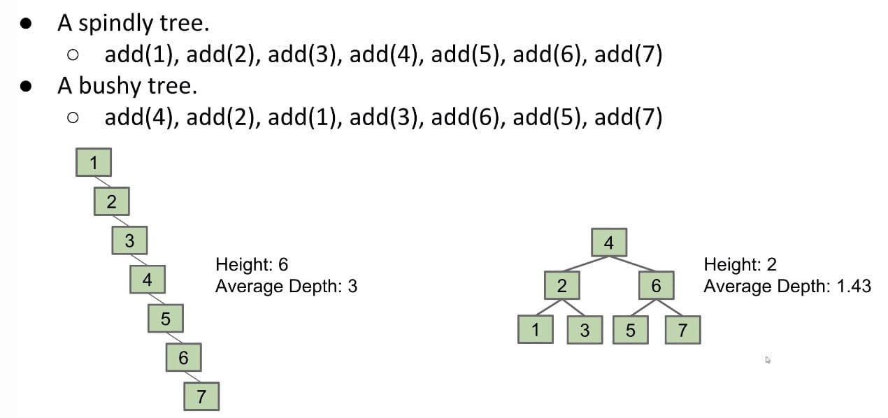
BST height is all four of these:
- $O(N)$
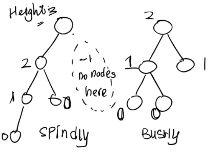
- $\Theta(\log{N})$ in the best case (“bushy”)
- $\Theta(N)$ in the worst case (“spindly”)
- $O(N^2)$ (technically true)
The middle two statements are more informative. Big-O is NOT mathematically the same thing as “worst case”, but it’s often used as shorthand for “worst case”.
Height and Depth
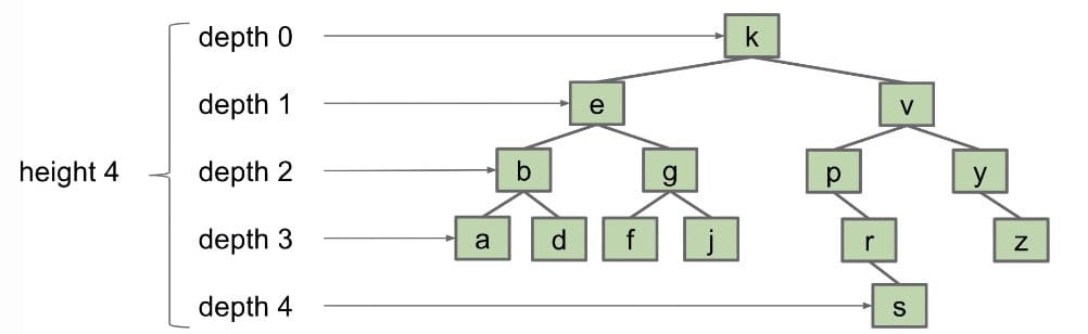
Depth: How far it is from the root, i.e. the number oflinksbetween a node and the root.Height: The lowest depth of a tree / The maximum depth of a tree.Average Depth: $\frac{\sum^D_{i=0}d_i n_i}{N}$ where $d_i$ is depth and $n_i$ is number of nodes at that depth.
The height of the tree determines the worst-case runtime, because in the worst case the node we are looking for is at the bottom of the tree. Similarly, the average depth determines the average-case runtime.
Orders matter!
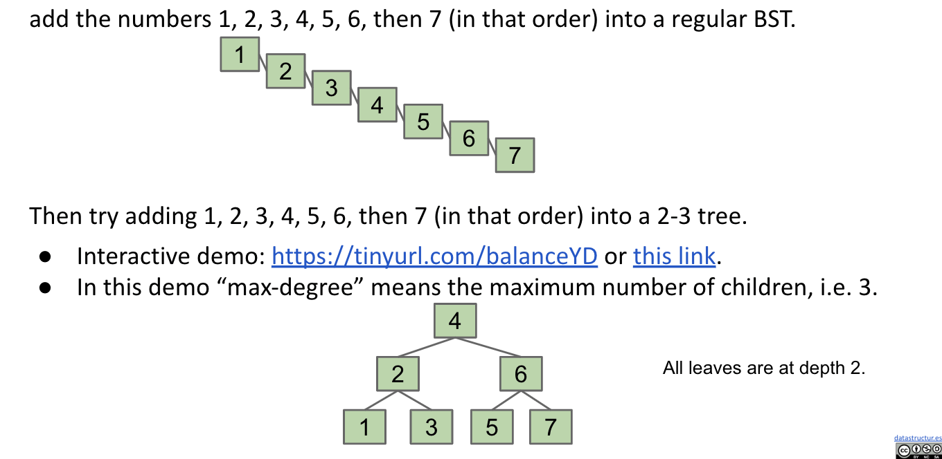
The order you insert nodes into a BST determines its height.
What about trees that you’d build during real world applications? One way to approximate this is to consider randomized BSTs.
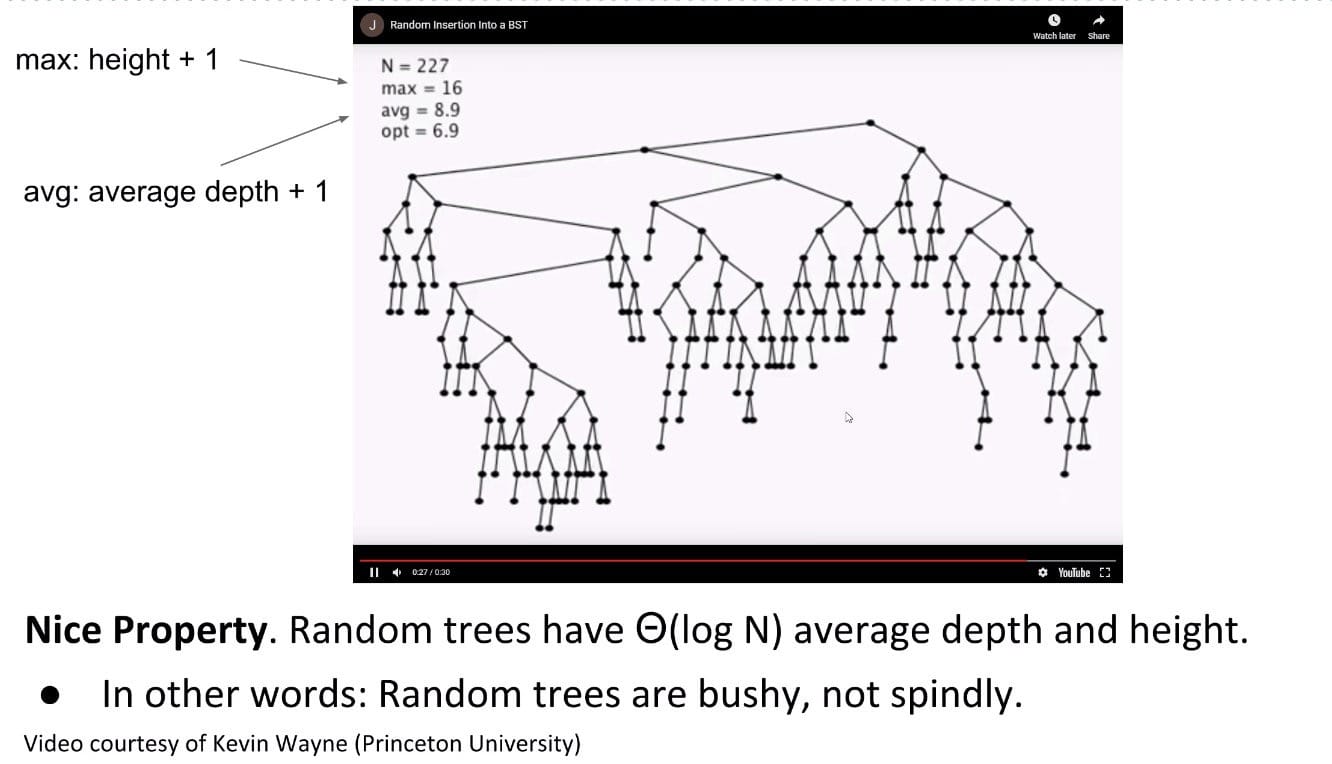
Therefore, Average Depth is expected to be $\sim 2 \ln{N} = \Theta(\log{N})$ with random inserts.
Note: $\sim$ is the same thing as Big Theta, but you don’t drop the multiplicative constants.
If $N$ distinct keys are inserted in random order, expected tree heights is $\sim 4.311 \ln{N}$. Thus, worst case runtime for contains operation is $\Theta(\log{N})$ on a tree built with random inserts.
Random trees including deletion are still $\Theta(\log{N})$ height.
Bad News:
The fact is that we can’t always insert our items in a random order, because data comes in over time, don’t have all at once (e.g. dates of events).
B-Trees
Also called 2-3, 2-3-4 Trees.
Crazy Idea
The problem with BST’s is that we always insert at a leaf node. This is what causes the height to increase.
Never add a leaf node!
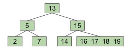
Solution: Set a limit on the number of elements in a single node. Let’s say 4. If we need to add a new element to a node when it already has 4 elements, we will split the node in half by bumping up the middle left node.
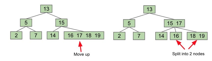
Notice that now the 15-17 node has 3 children now, and each child is either less than, between, or greater than 15 and 17.
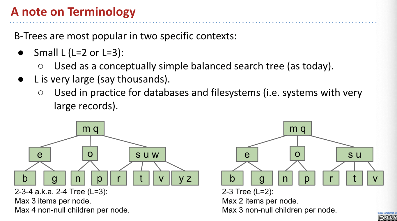
These trees are called B-trees or 2-3-4/2-3 Trees. 2-3-4 (L=3) and 2-3 (L=2) refer to the number of children each node can have. So, a 2-3-4 tree can have 2, 3, or 4 children while a 2-3 tree can have 2 or 3.
- 2-node: has 2 children.
- 3-node: has 3 children.
- 4-node: has 4 children.
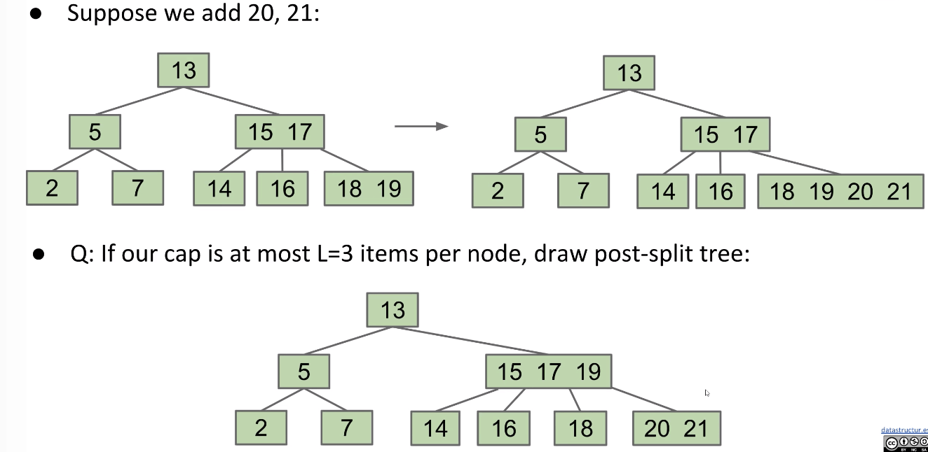
This means that 2-3-4 trees split nodes when they have 3 nodes (4 children) and one more needs to be added. 2-3 trees split after they have 2 nodes (3 children) and one more needs to be added.
Adding a node to a 2-3-4 tree:
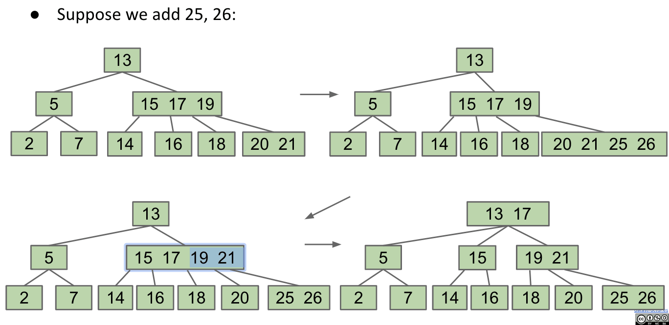
- After adding the node to the leaf node, if the new node has 4 nodes, then pop up the
middle-leftnode and re-arrange the children accordingly. - If this results in the parent node having 4 nodes, then pop up the middle left node again, rearranging the children accordingly.
- Repeat this process until the parent node can accommodate or you get to the root.
Add: Chain Reaction
What Happens If The Root Is Too Full?
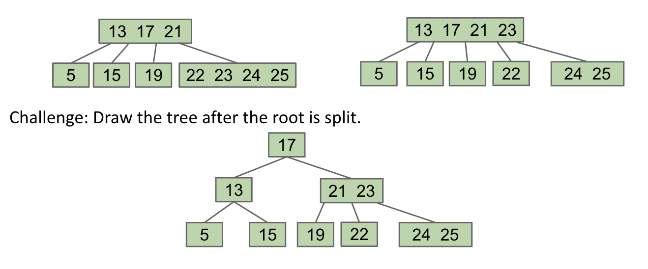
Observation: Splitting-trees (B-trees) have perfect balance.
- If we split the root,
every nodegets pushed down by exactly one level. - If we split a leaf node or internal node, the height doesn’t change.
The origin of “B-tree” has never been explained by the authors. As we shall see, “balanced,” “broad,” or “bushy” might apply. Others suggest that the “B” stands for Boeing. Because of his contributions, however, it seems appropriate to think of B-trees as “Bayer”-trees.
– Douglas Corner (The Ubiquitous B-Tree)
B-Trees Usage:
B-Trees are most popular in two specific contexts:
- Small $L$ ($L = 2$ or $L = 3$)
- Used as a conceptually simple balanced search tree.
- Very large $L$ (say thousands)
- Used in practice for databases and file systems.
Invariants
Interactive demo: link
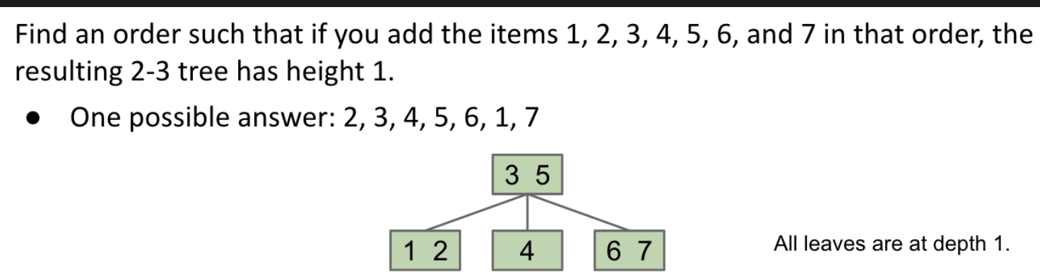
No matter the insertion order you choose, resulting B-Tree is always bushy.
Why?
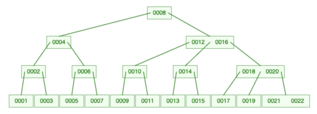
Because of the way B-Trees are constructed (growing from the root), we get two nice invariants:
- All leaves must be the
same distancefrom the source. (growing from the root & growing horizontally) - A non-leaf node with $k$ items must have exactly $k + 1$ children. ($k + 1$ gaps between items)
These invariants guarantee that trees are bushy.
Runtime Analysis
Height
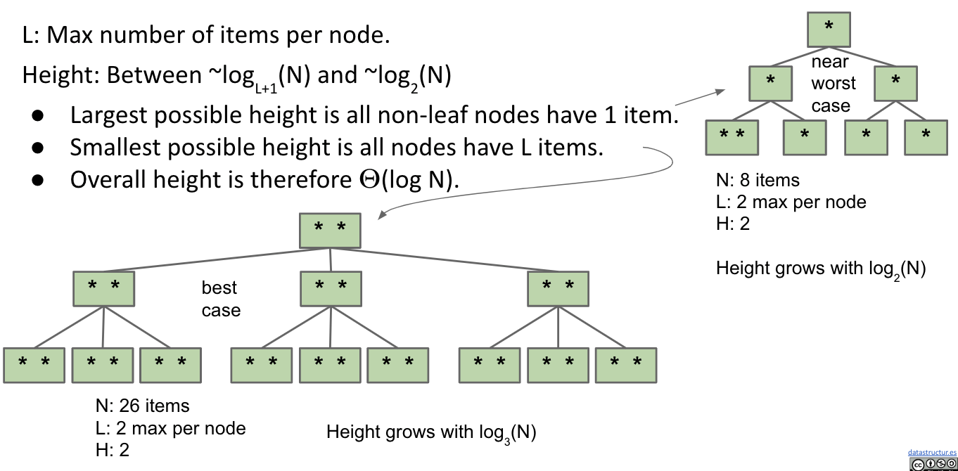
Thus, the height is between $\sim\log_{L+1}{(N)}$ and $\sim\log_2{(N)}$
More items in a node => More branches => More stuff for the same height
contains
- Worst case number of nodes to inspect: $H+1$
- Worst case number of items to inspect per node: $L$
- Overall runtime: $O(HL) = O(\log{N})$
- Since $H = \Theta(\log{N})$, overall runtime is $O(L\log{N})$.
- Since $L$ is a constant, runtime is therefore $O(\log{N})$.
add
It is similar to contains.
- Worst case number of nodes to inspect: $H+1$
- Worst case number of items to inspect per node: $L$
- Worst case number of split operations: $H+1$
- Overall runtime: $O(HL) = O(L)$
So, runtime is $O(\log{N})$.
B-trees are more complex, but they can efficiently handle any insertion order.
deletion
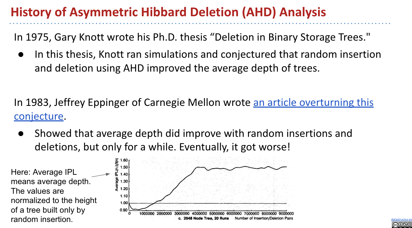
History
Random Insertions & Deletions in BST:
$O(\sqrt{N})$ / $\Theta(\log{N^2})$ average height after random insertions and deletions. Assumes you always pick the successor when deleting!
History:
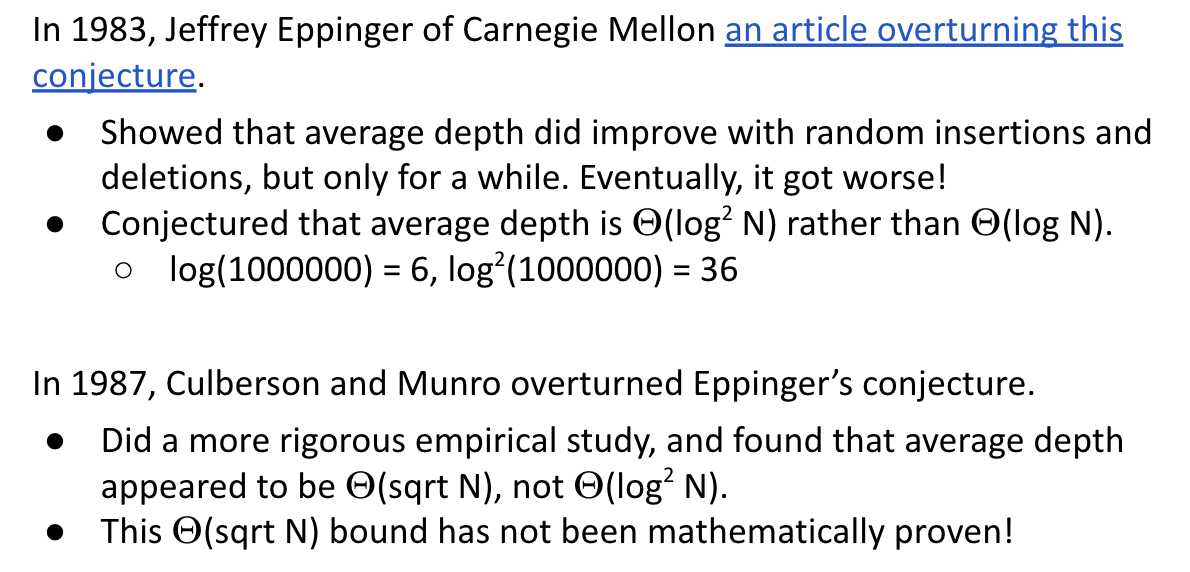
But, if you randomly pick between successor and predecessor, you get $\Theta(\log{N})$ height.
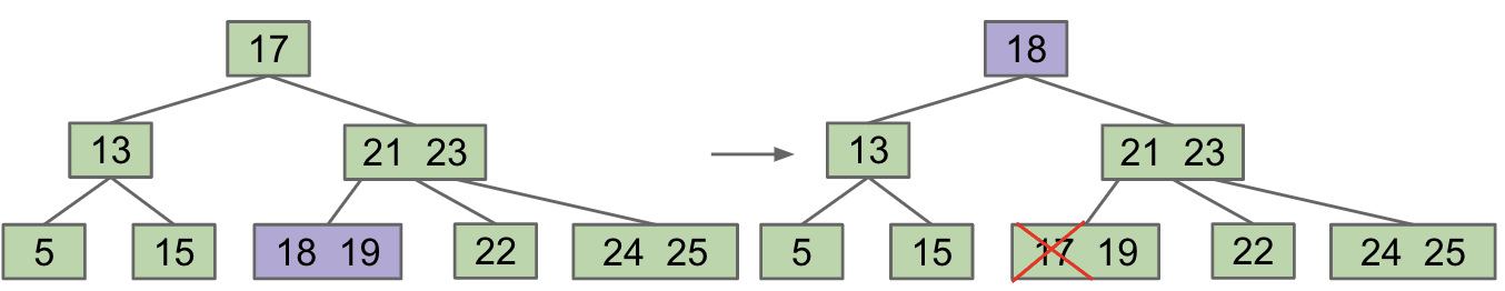
2-3 Deletion
There are many possible deletion algorithms.
In a 2-3 Tree, when we delete $\alpha$ from a node with two or more children, we:
Swapthe value of the successor with $\alpha$- Then we
deletethe successor value (always be in a leaf node, because the tree is bushy!)
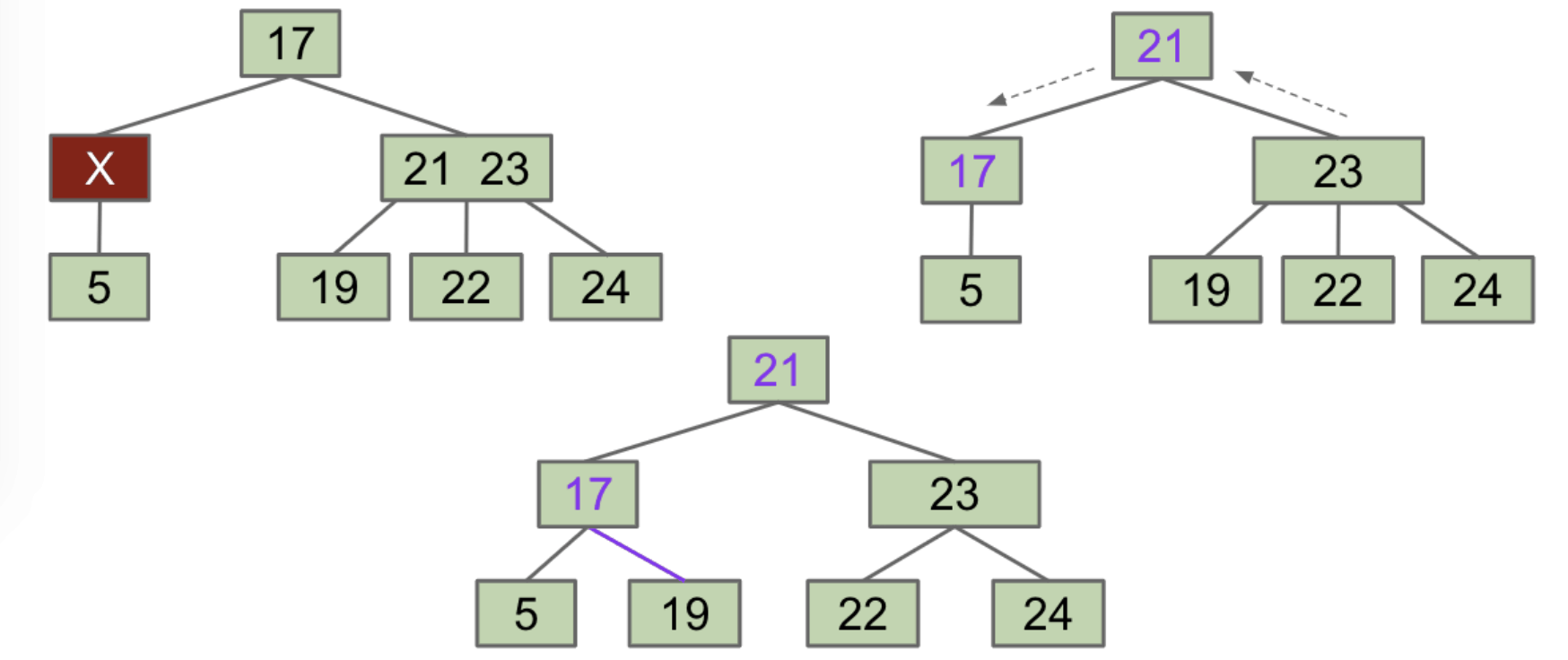
Example: delete(17)
If the leaf has multiple keys, the deletion is trivial. Just simply remove the item. What about Single-Key Leaves?
We need to keep the invariants (Any node with k items must have k + 1 children!). So, we’ll leave an empty node, which must be filled.
Note: It depends on the number of parent keys and sibling keys.
Filling in Empty Nodes (FIEN)
The hard part about deletion in 2-3 Trees is filling empty nodes.
FIEN Case 1A:
Multi-Key Sibling- $X$ steals parent’s item. Parent steals sibling’s item.
- If $X$ was not a leaf node, $X$ steals one of sibling’s subtrees.
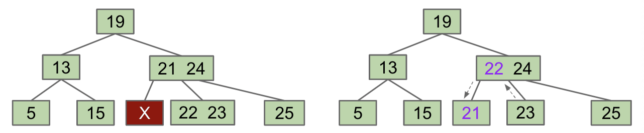
Another example: Try to delete 17 from the tree below.
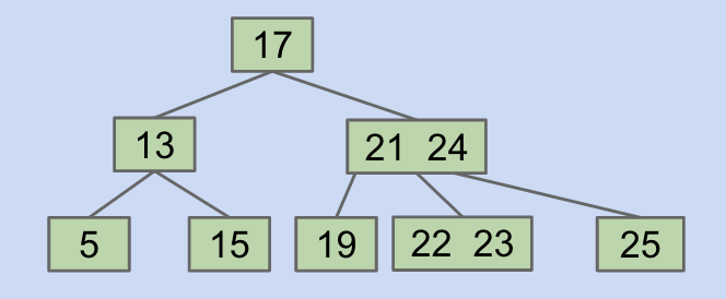
Answer:
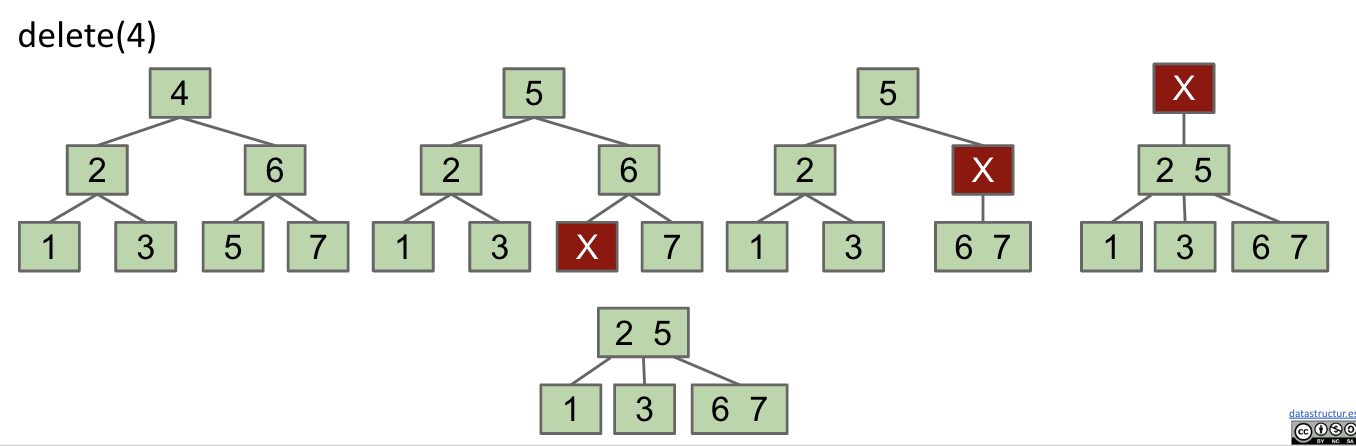
FIEN Case 2A:
Multi-Key Parent- $X$ and right sibling steal parent’s keys.
Middle siblingmoves into the parent. - Subtrees are passed along so that every node has the correct children.
Another example: Try to delete root 3
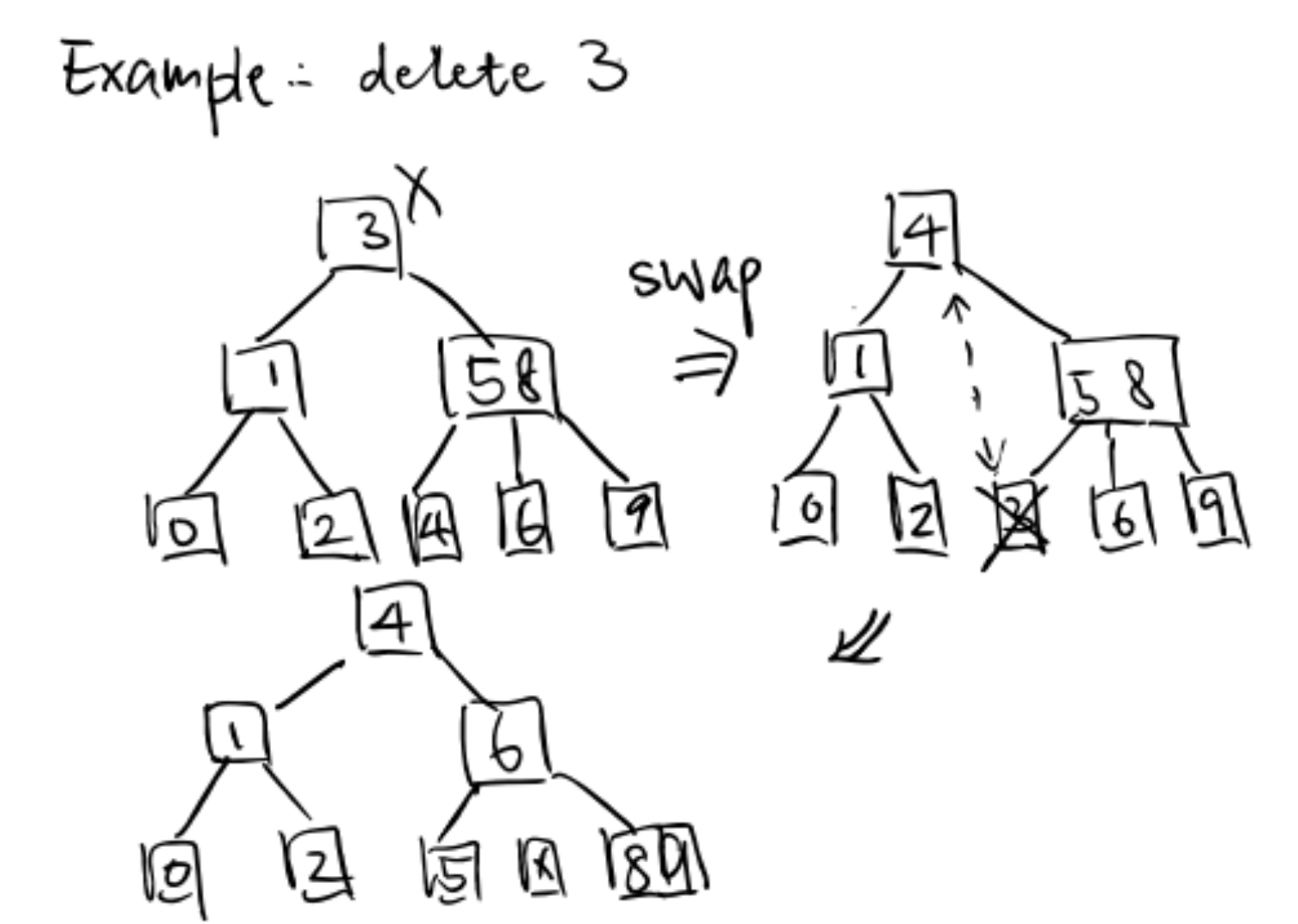
- $X$ and right sibling steal parent’s keys.
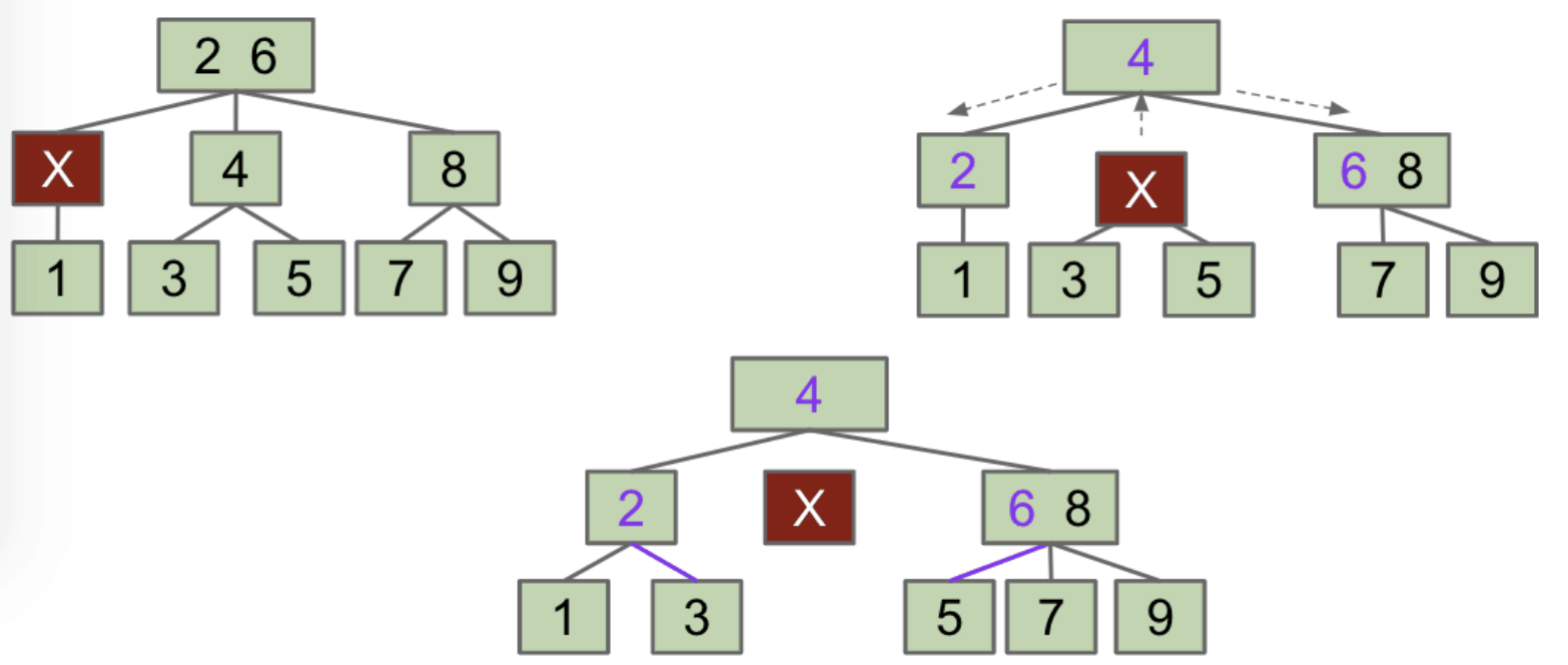
FIEN Case 3:
Single-Key Parent and Sibling- Combine 1 sibling and parent into a single node that replaces $X$. Send the blank $X$ up one level.
- If blank ends up as the new root, just delete the blank and we are done.
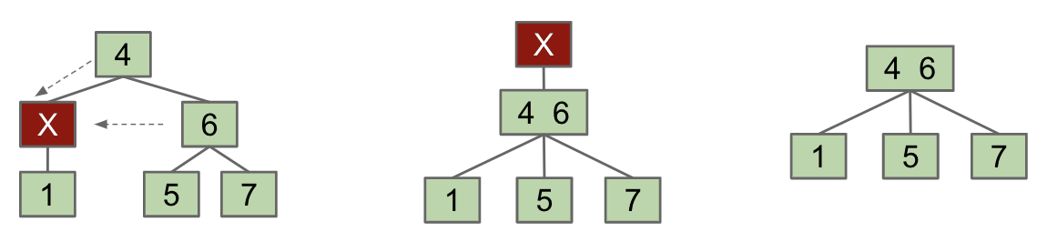
Exercise 1: Delete 6
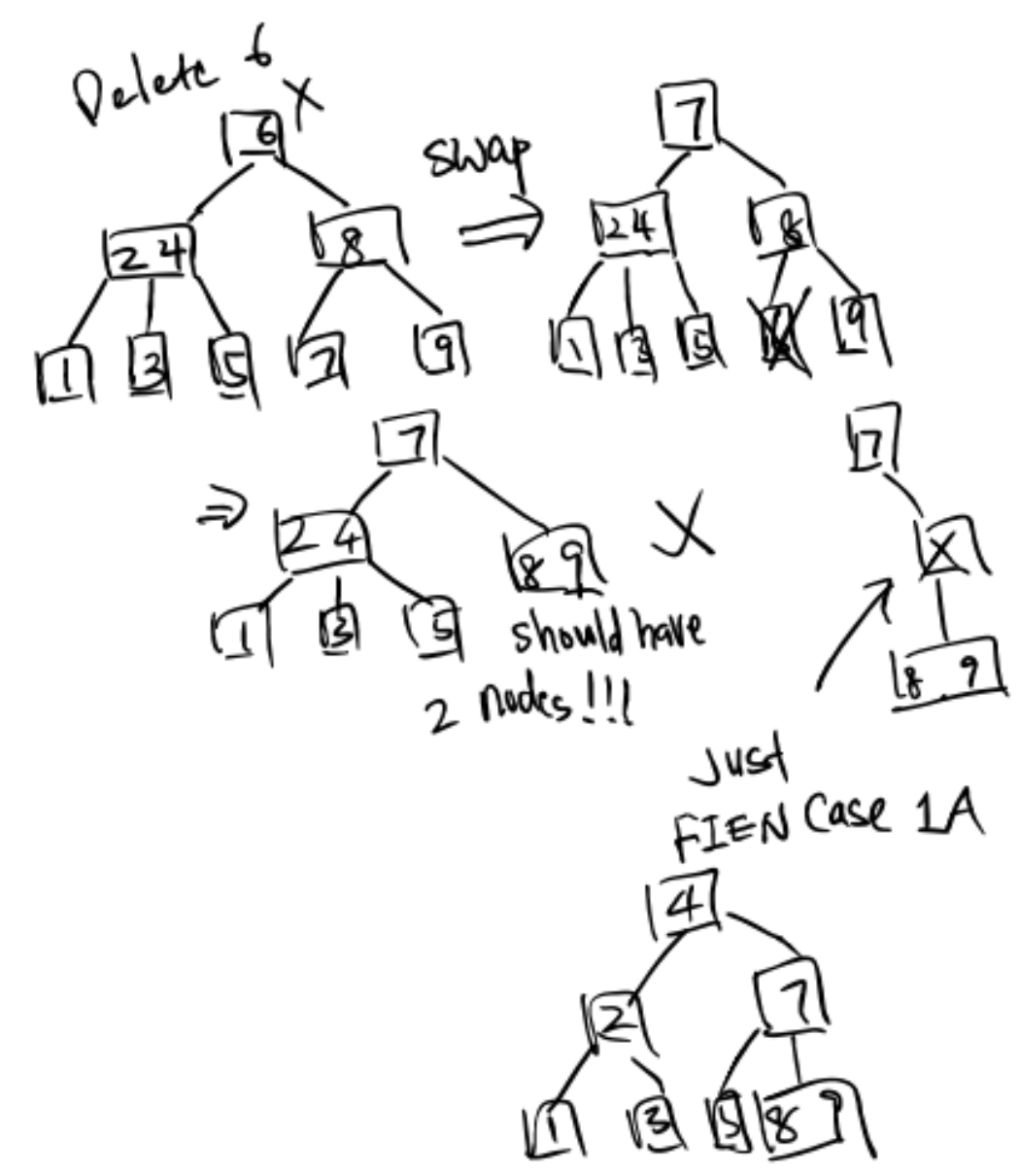
Exercise 2: Delete 4
Notice that the combination is recursive.
Implementation
My implementation: MyBTree.java
Algs4: BTree.java (I don’t quite understand the code)
Ex (Guide)
The key idea of a B-Tree is to over stuff the nodes at the bottom to prevent increasing the height of the tree. This allows us to ensure a max height of $\log{N}$.
Ex 1
Problem 5 of the Fall 2014 midterm.
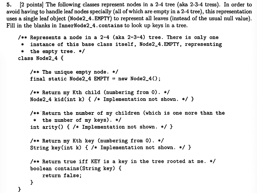
1 | class InnerNode2_4 extends Node2_4 { |
Ex 2
Problem 1c, e of the Spring 2018 Midterm 2
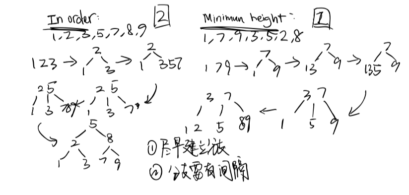
Draw a valid B-Tree of minimum height containing the keys 1, 2, 3, 7, 8, 5.
In Order: 1, 2, 3, 5, 7, 8, 9
Drawing sequence: 1, 7, 9, 3, 5, 2, 8
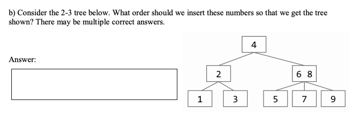
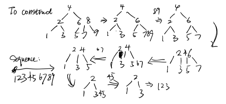
Ex 3
Problem 8b of the Spring 2016 Midterm 2
Tree Rotation
Issues of B-Trees
Wonderfully balanced as they are, B-Trees are really difficult to implement. We need to keep track of the different nodes and the splitting process is pretty complicated. As computer scientists who appreciate good code and a good challenge, let’s find another way to create a balanced tree.
Issues:
- Maintaining different node types
- Interconversion of nodes between 2-nodes and 3-nodes
- Walking up the tree to split nodes
1 | // put method of B-Tree |
Beautiful algorithms are, unfortunately, not always the most useful. - Knuth
Rotation
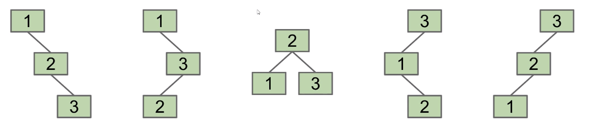
Given any BST, it is possible to move to a different configuration using “rotation”.
More generally, for $N$ items, there are Catalan(N) (number of states of many recursive data structures) different BSTs.
In general, we can move from any configuration (bushy tree) to any other in 2n - 6 rotations.
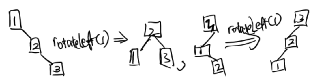
The formal definition of rotation is:
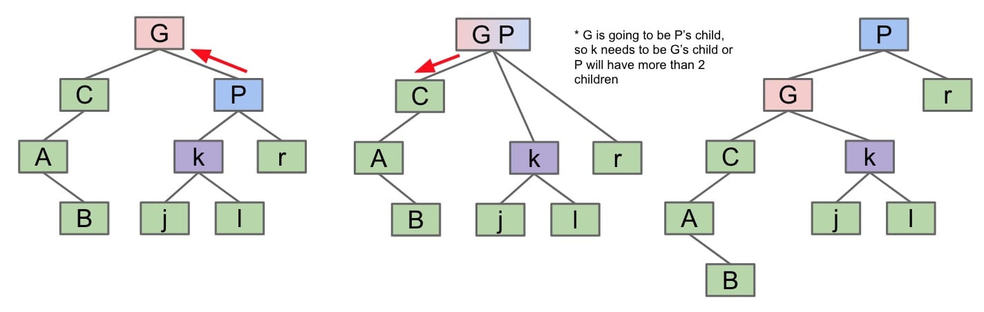
rotateLeft(G): Let $x$ be the right child of $G$. Make $G$ the new left child of $x$. (also assign $P$’s left child to $G$ as its right child)
- Alternatively, merging $G$ and $P$, then sending $G$ down and left.
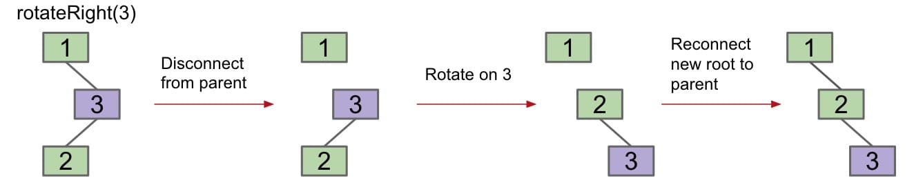
rotateRight(G): Let $x$ be the left child of $G$. Make $G$ the new right child of $x$.
Practice: (make it bushy)
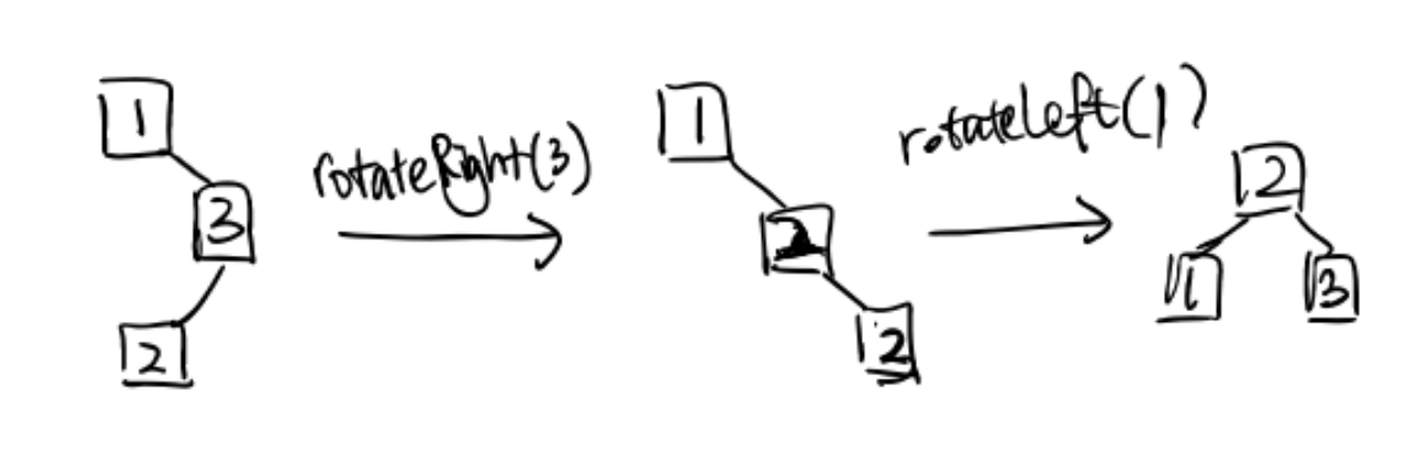
Note: In the middle case, rotate(3) is undefined.
Usage:
- Can shorten (or lengthen) a tree.
- Preserves search tree property.
Code:
1 | private TreeNode rotateRight(TreeNode x) { |
Red Black Trees
LLRB Definition
So far, we’ve encountered two kinds of search trees:
- BST: Can be balanced by using rotation.
- 2-3 Trees: Balanced by construction, i.e. no rotations required.
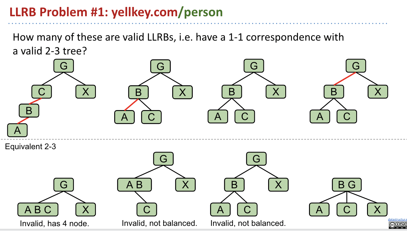
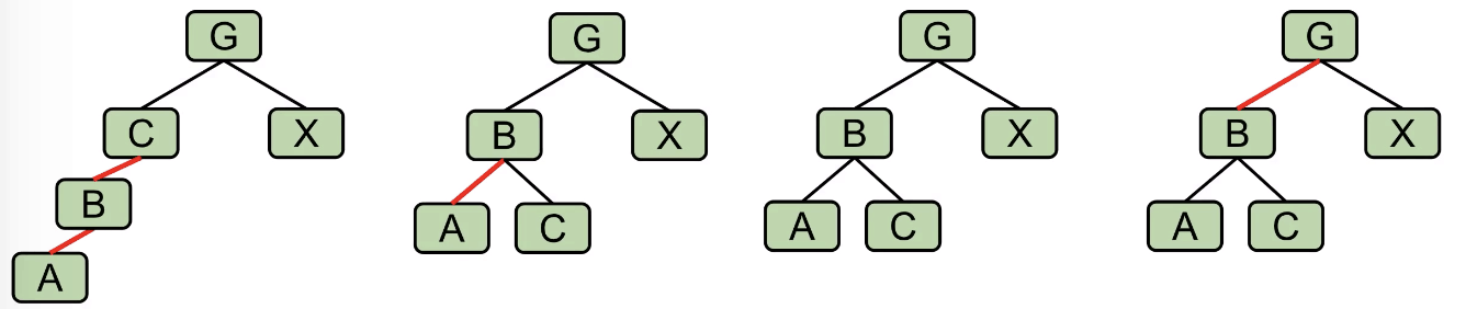
Goal: Build a BST that is structurally identical to a 2-3 tree.
Left-Leaning Red Black trees have a 1-1 correspondence with 2-3 trees.
- Every 2-3 tree has a unique
LLRB Red Blacktree associated with it. - As for 2-3-4 trees, they maintain correspondence with
standard Red Black trees.
Possibility 1: Create dummy “glue” nodes
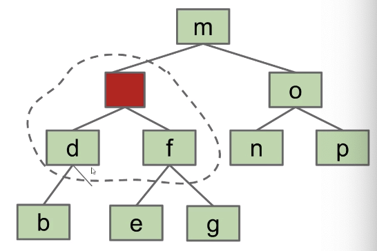
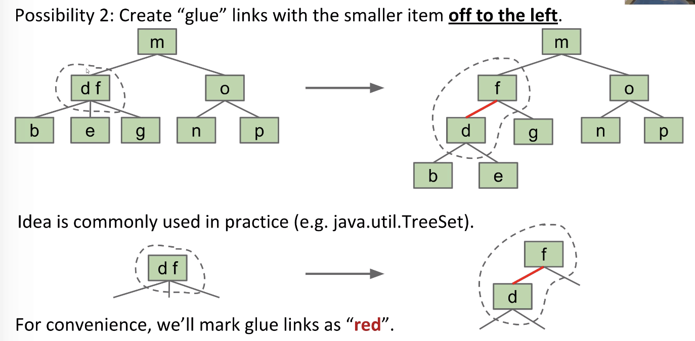
Possibility 2: Create “glue” links with the smaller item off to the left
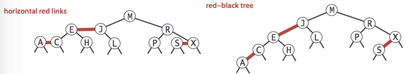
LLRB Properties
Left-Leaning Red Black Binary Search Tree (LLRB)
A BST with left glue links that represents a 2-3 tree is often called an LLRB (BST is omitted).
- There is a
1-1correspondence between an LLRB and an equivalent 2-3 tree. - The
red linksare just a convenient fiction. Red links don’t “do” anything special. They connect nodes within a 3-node. - The
black linksconnect 2-nodes or 3-nodes.
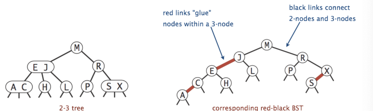
Consider what an LLRB might look like:
Note: Each 3-node becomes two nodes in the LLRB. So, in terms of height, an LLRB has no more than ~2 times the height of its 2-3 tree.
The worst case is that along the path each node is 3-node (~2 times in the worst case).
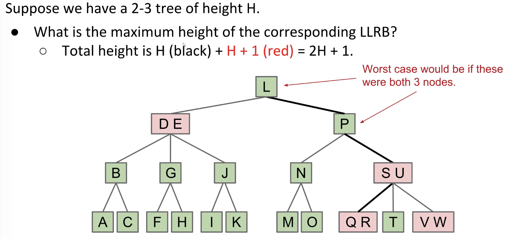
Maximum comparison: $2H + 2$.
Some handy LLRB properties:
- No node has
two red linksincluding the link to its parent (up) and links to children (down). Otherwise it’d be analogous to a 4-node. Every pathfrom root to a leaf hassame number of black links, because 2-3 trees have the same number of links to every half (only number of red links vary). Therefore, LLRBs are balanced.
Important Idea of Runtime:
We know an LLRB’s height is no more than around double the height of its 2-3 tree. Since the 2-3 tree has the height that is logarithmic in the number of items, the LLRB is also logarithmic in the number of items.
One last question: Where do LLRBs come from?
It turns out we implement the LLRB insertion as follows:
- Insert as usual into a BST.
- Use
0 or more rotationsto maintain the 1-1 mapping.
Maintain LLRB
Implementation of an LLRB is based on maintaining this 1-1 correspondence.
- When performing LLRB operations,
pretendlike you’re a 2-3 tree. - Preservation of the correspondence will involve tree rotations.
Task #1: Insertion Color
Should we use a red or black link when inserting?
Use RED! In 2-3 trees, new values are ALWAYS added to a leaf node (at first).
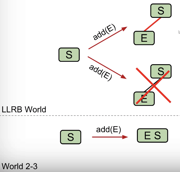
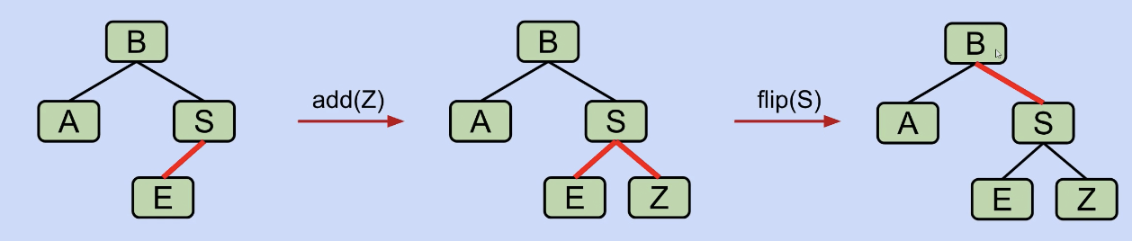
Task #2: Insertion on the Right
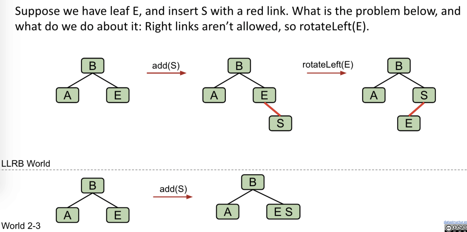
Right links aren’t allowed (because it is an LLRB). Use rotation. If we add one more node, we’ll have 2 red links.
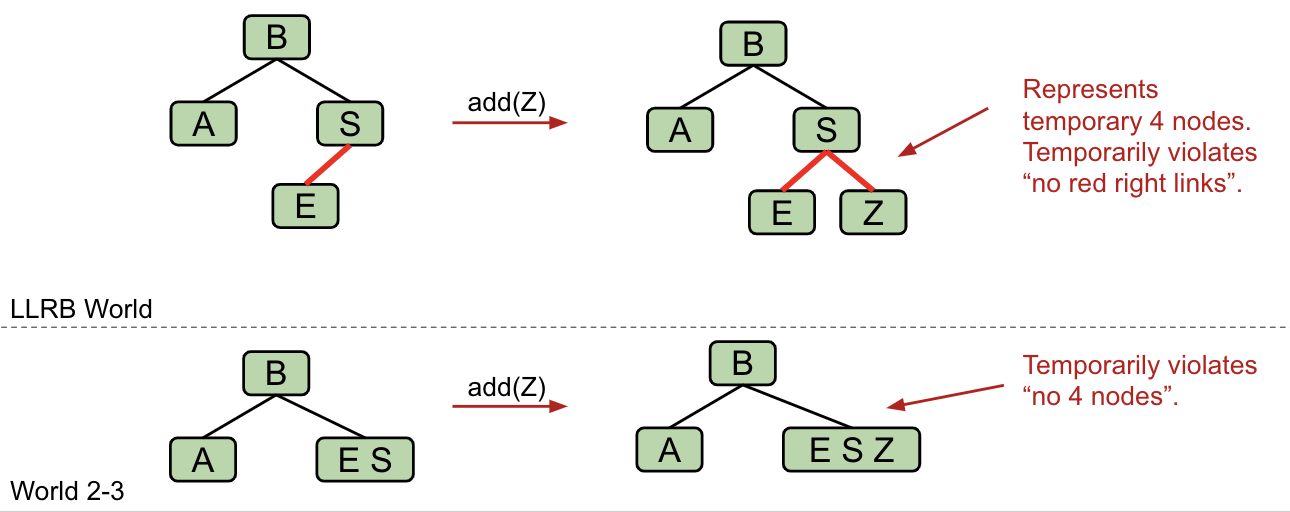
New Rule: We need to represent the temporary 4-nodes.
We will represent temporary 4-nodes as BST nodes with two red links. This state is only temporary, so temporary violation of “left leaning” is OK.
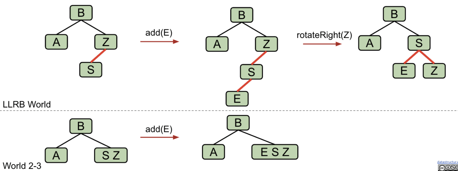
Task #3: Double Insertion on the Left
Suppose we have the LLRB below and insert $E$. We end up with the wrong representation for our temporary 4-node. We need to do some rotations.
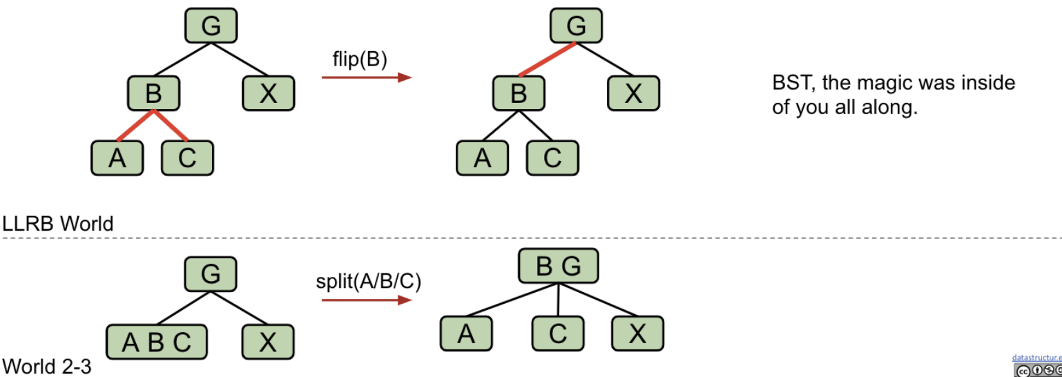
Task #4: Splitting Temporary 4-Nodes
Suppose we have the LLRB below which includes a temporary 4-node. Flip the color of all edges touching B.
Summary
- When inserting:
- Use a
red link.
- Use a
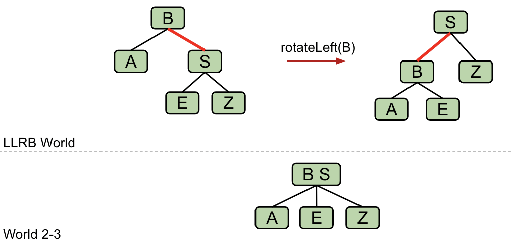
- If there is a right leaning “3-node”, it violates the
left-leaning violation.Rotate leftthe appropriate node to fix.
- If there are two consecutive left links, it violates the
incorrect 4-node violation.Rotate rightthe appropriate node to fix.
- If there are any nodes with two red children, we have a
temporary 4-node.Color flipthe node to emulate the split operation.
One last detail: Cascading operations (Just like 2-3 tree operations).
- It is possible that a rotation or flip operation will cause an additional violation that needs fixing.
For example:
Exercise:
Answer: link (my drawing)
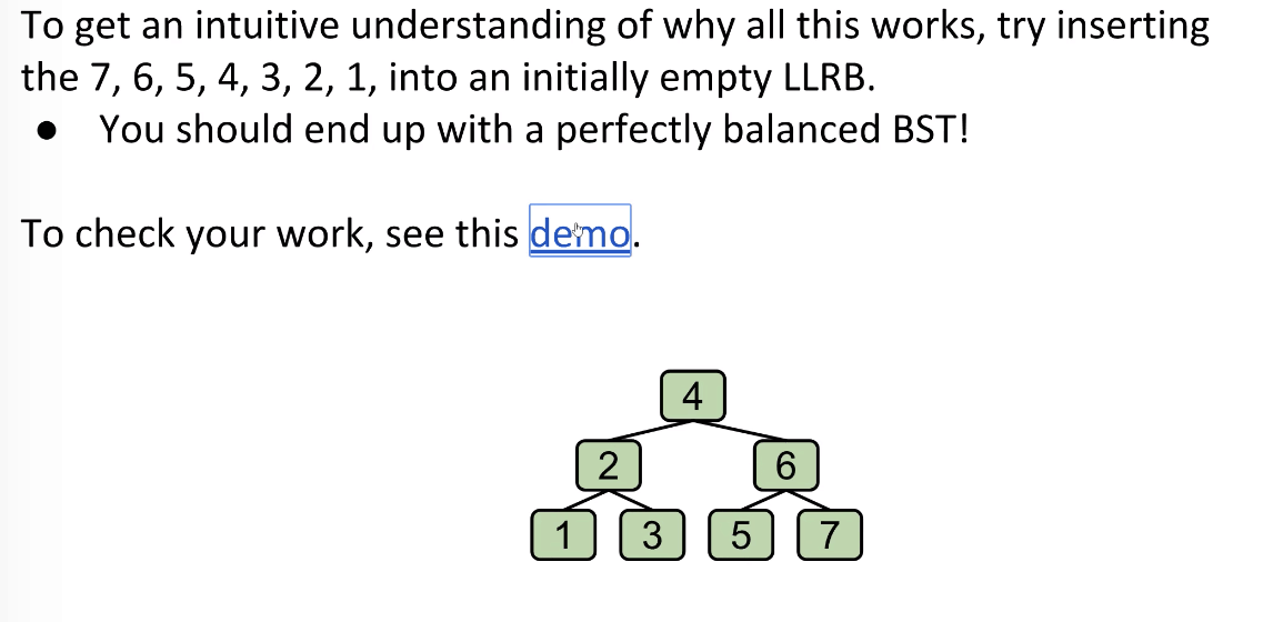
What about inserting 1 through 7?
Answer: link (my drawing)
Implementation
Insert is $O(\log{N})$:
- $O(\log{N})$: Add the new node.
- $O(\log{N})$: Rotation and color flip operations per insert.
Turning a BST into an LLRB requires only 3 clever lines of code.
1 | // How to represent RED? |
Java’s TreeMap is a red black tree (not left-leaning).
- Maintain correspondence with 2-3-4 tree (not a 1-1 correspondence).
- Allow glue links on either side.
- More complex implementation, but significantly faster.
There are many other types of search trees out there. Other self-balancing trees: AVL trees, splay trees, treaps, etc (at least hundreds of them).
And there are other efficient ways to implement sets and maps entirely.
- Other linked structures:
Skip listsare linked lists with express lanes. - Other ideas entirely:
Hashingis the most common alternative.
Skip List
Skip List | Set 1 (Introduction)
Question: Can we search in a sorted linked list (a sorted array can apply Binary Search because of random access) in better than $O(n)$ time?
Idea: Create multiple layers so that we can skip some nodes.
The upper layer works as an express lane which connects only main outer stations, and the lower layer works as a normal lane which connects every station.
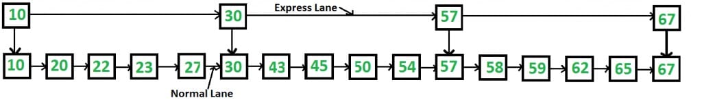
Suppose we want to search for 50, we start from first node of “express lane” and keep moving on “express lane” till we find a node whose next is greater than 50.
What is the time complexity with two layers?
The worst case time complexity is number of nodes on “express lane” plus number of nodes in a segment (nodes between adjacent two “express lane” nodes). Suppose we have $n$ nodes on “normal lane”, $\sqrt{n}$ nodes on “express lane”, and we equally divide the “normal lane”, then there will be $\sqrt{n}$ nodes in every segment (interesting).
Actually, $\sqrt{n}$ is the optimal division with two layers. With this arrangement, the number of nodes traversed for a search will be $O(\sqrt{n})$.
Can we do better?
The time complexity of skip lists can be reduced further by adding more layers. In fact, the time complexity of search, insert and delete can become $O(\log{n})$ in average case with $O(n)$ extra space.
Another Idea: Self Organizing List
Self Organizing List | Set 1 (Introduction)
Self Organizing List is to place more frequently accessed items close to head. There can be two possibilities:
offline: We know the complete search sequence in advance.online: We don’t know the search sequence.
In case of offline, we can put the nodes according to decreasing frequencies of search, which means that the element having maximum search count is put first.
Following are different strategies used by Self Organizing Lists:
- Move-to-Front Method
- Count Method
- Transpose (Swap) Method
The worst case time complexity of all methods is $O(n)$. In worst case, the searched element is always the last element in list. For average case analysis, we need probability distribution of search sequences which is not available many times.
AVL Trees
They are self-balancing search trees.
Definition: AVL (named after inventors Adelson-Velsky and Landis) tree is a self-balancing Binary Search Tree (BST) where the difference between heights of left and right subtrees cannot be more than one for all nodes.
Why log N?
The AVL tree always has at most 1-level difference between child subtrees for all nodes. If the difference is so big, you can imagine all nodes grow on the left side of a tree, which then increases the height of a tree.
Since the tree looks bushy with this constraint, the height of the AVL tree is $\log{N}$ and is balanced.
Further, insertion takes $O(\log{N})$. Every time a node is added to the AVL tree, you need to update the height of the parents all the way up to the root. Since the tree is balanced, updating heights will traverse only the linked-list structure with the newly inserted node in the tail, which takes also $O(\log{N})$.
AVL trees height proof (optional)
AVL Rules
AVL Trees & Where To Find (Rotate) Them
- A tree is height-balanced when the heights of its two subtrees differ by at most $1$.
- The
balance factoris defined as an integer in the range of $\left[-1, 1\right]$ where $-1$ indicates that there is an extra node on the right subtree’s path of maximum depth.- $balance\ factor = H_{left\ subtree} - H_{right\ subtree}$
- A tree is considered
unbalancedwhen the balance factor falls outside that range, say $-2$ or $2$.
Insert
Idea
Let the newly inserted node be $w$:
- Perform standard BST insert for $w$.
- Starting from $w$,
travel upand find the first unbalanced node, e.g. $z$ with thechild$y$ andgrandchild$x$ along the path.1
2
3
4
5
6
7
8// alphabet order: u v w x y z
z -- height: 3
/ \
y T4 -- height: 2 & 0, factor = 2
/ \
x T3
/ \
T1 T2 - Re-balance the tree by
performing appropriate rotationson the subtree rooted with $z$. There can be four possible cases that need to be handled:- Left-Left (LL) => Single Right Rotation
1
2
3
4
5
6
7
8
9// [z] is the unbalanced node.
T1, T2, T3 and T4 are subtrees.
[z] y
/ \ / \
y T4 Right Rotate [z] x z
/ \ - - - - - - - - -> / \ / \
x T3 T1 T2 T3 T4
/ \
T1 T2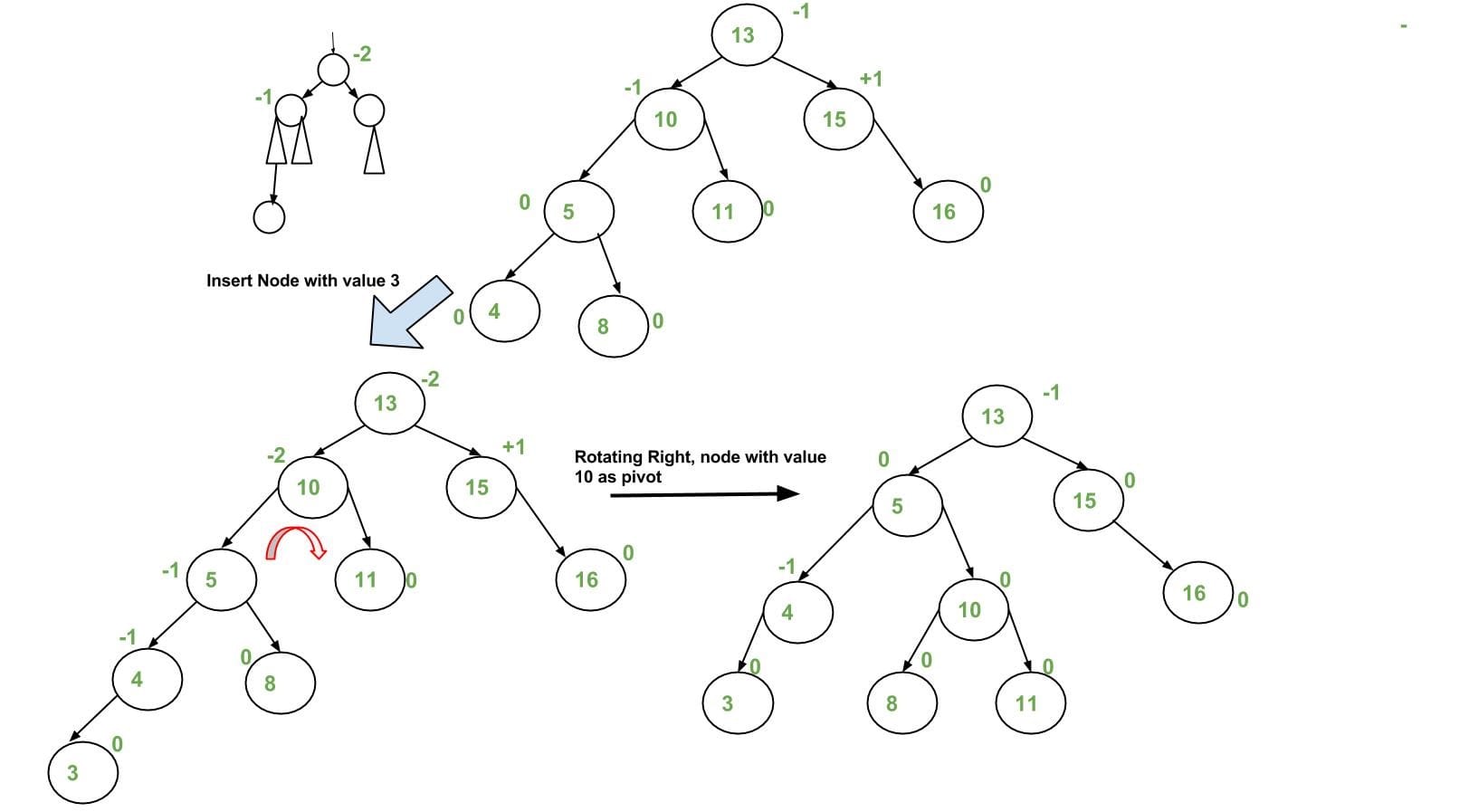
Note: The example uses difference between left-subtree’s height and right-subtree’s height. - Left-Right (LR) => Double Left-Right Rotation
Left Rotatey(pivot) => Change it to Left-Left case
Right Rotatez(root)1
2
3
4
5
6
7
8// [z] is the unbalanced node.
z [z] x
/ \ / \ / \
[y] T4 Left Rotate [y] x T4 Right Rotate [z] y z
/ \ - - - - - - - - > / \ - - - - - - - -> / \ / \
T1 x y T3 T1 T2 T3 T4
/ \ / \
T2 T3 T1 T2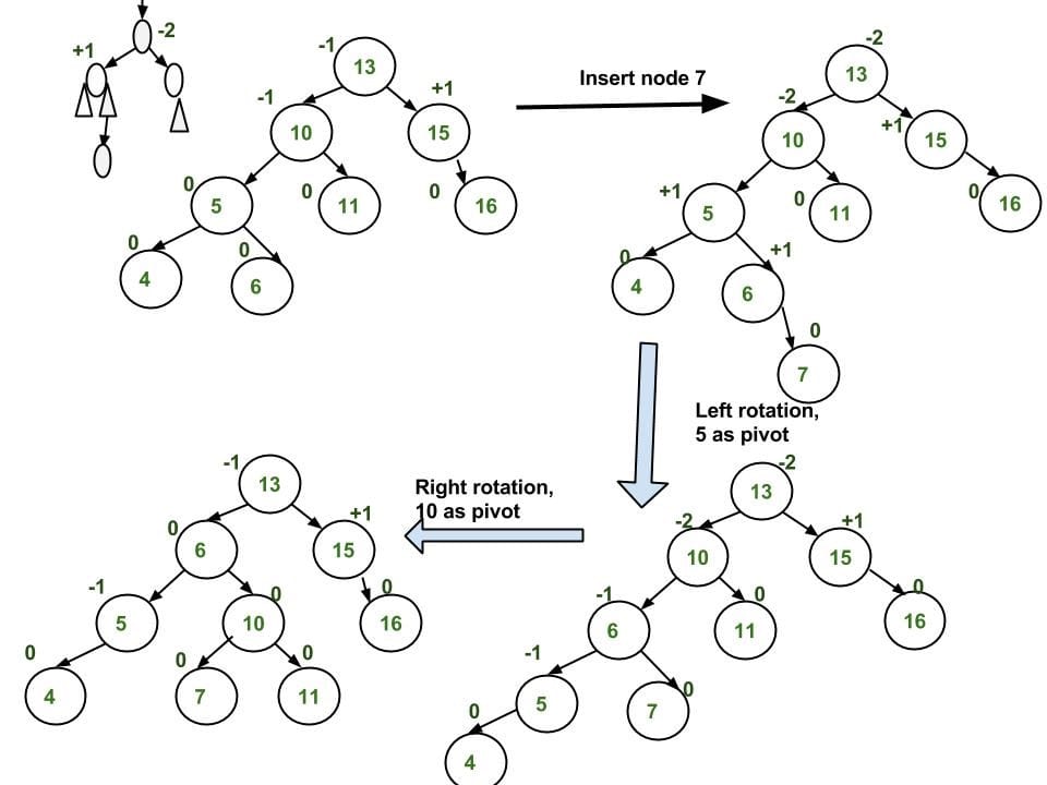
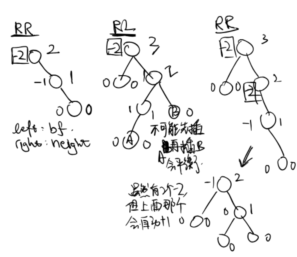
- Right-Right (RR) => Single Right Rotation
1
2
3
4
5
6
7[z] y
/ \ / \
T1 y Left Rotate [z] z x
/ \ - - - - - - - -> / \ / \
T2 x T1 T2 T3 T4
/ \
T3 T4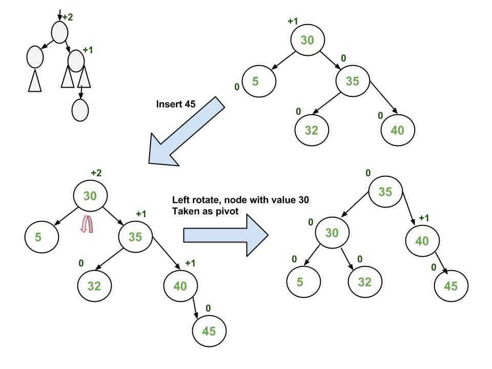
- Right-Left (RL) => Double Right-Left Rotation
1
2
3
4
5
6
7z [z] x
/ \ / \ / \
T1 [y] Right Rotate [y] T1 x Left Rotate [z] z y
/ \ - - - - - - - - -> / \ - - - - - - - -> / \ / \
x T4 T2 y T1 T2 T3 T4
/ \ / \
T2 T3 T3 T4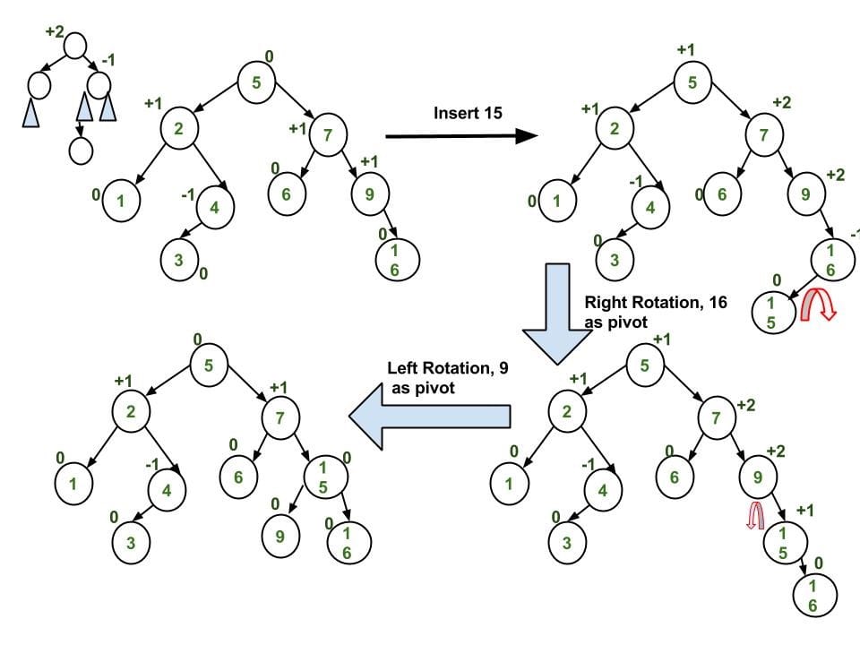
- Left-Left (LL) => Single Right Rotation
Implementation
- Perform the normal BST insertion.
- The current node must be one of the
ancestorsof the newly inserted node. Update the height of the current node. - Get the
balance factor(left subtree height - right subtree height) of the current node.- If
balance factoris greater than $1$, the current node is unbalanced and we have either LL or LR case.- The
balance factorof the left subtree < 0 => LR - Or, compare the newly inserted key with the key in left subtree root.
- The
- If
balance factoris less than $-1$, the current node is unbalanced and we have either RR or RL case.- The
balance factorof the right subtree > 0 => RL - Or, Compare the newly inserted key with the key in right subtree root.
- The
- If
Code
Reference: algs4 - AVLTreeST.java
Insert / Put
1
2
3
4
5
6
7
8
9
10
11
12
13
14
15
16
17
18
19
20
21
22
23
24
25
26public void put(Key key, Value val) {
if (key == null) throw new IllegalArgumentException("first argument to put() is null");
if (val == null) {
delete(key); return;
}
root = put(root, key, val);
assert check();
}
private Node put(Node x, Key key, Value val) {
if (x == null) {
return new Node(key, val, 0, 1); // with height 0 and size 1
}
int cmp = key.compareTo(x.key);
if (cmp < 0) {
x.left = put(x.left, key, val);
} else if (cmp > 0) {
x.right = put(x.right, key, val);
} else { /* found & update */
x.val = val;
return x;
}
x.size = 1 + size(x.left) + size(x.right);
x.height = 1 + Math.max(height(x.left), height(x.right));
return balance(x); // the magic is here
}Balancing Methods:
1
2
3
4
5
6
7
8
9
10
11
12
13
14
15
16
17
18
19
20
21
22
23
24
25
26private Node balance(Node x) {
int bf = balanceFactor(x);
// balanced
if (bf <= 1 || bf >= -1) {
return x;
}
// LL, LR
if (bf(x) > 1) {
if (bf(x.left) < 0) { // or if (key > x.left.key)
x.left = rotateLeft(x.left); // LR
}
x = rotateRight(x); // LL
}
// RR, RL
if (bf(x) < -1) {
if (bf(x.right) > 0) { // or if (key < x.right.key)
x.right = rotateRight(x.right); // RL
}
x = rotateLeft(x); // RR
}
return x;
}
private int balanceFactor(Node x) {
return height(x.left) - height(x.right);
}Rotation
1
2
3
4
5
6
7
8
9
10
11
12
13
14
15
16
17
18
19
20
21
22
23
24
25
26
27private Node rotateRight(Node x) {
// notice the order
Node h = x.left; // new boss
x.left = h.right;
h.right = x;
// update sizes
h.size = x.size; // new boss
x.size = 1 + size(x.left) + size(x.right);
// update heights
x.height = 1 + Math.max(height(x.left), height(x.right));
h.height = 1 + Math.max(height(h.left), height(h.right));
return h;
}
private Node rotateLeft(Node x) {
// notice the order
Node h = x.right; // new boss
x.right = h.left;
h.left = x;
// update sizes
h.size = x.size; // new boss
x.size = 1 + size(x.left) + size(x.right);
// update heights;
x.height = 1 + Math.max(height(x.left), height(x.right));
h.height = 1 + Math.max(height(h.left), height(h.right));
return h;
}
AVL vs. Red Black
The AVL tree and other self-balancing search trees like Red Black trees are useful to get all basic operations done in $O(\log{N})$ time. The AVL trees are more balanced compared to Red Black trees, but they may cause more rotations during insertion and deletion.
- So if your application involves many frequent insertions and deletions, then
Red Black treesshould be preferred. - And if the insertions and deletions are less frequent and search is the more frequent operation, then
AVL treesshould be preferred over Red Black trees.
Delete
Similar processes to insertion. But note that, unlike insertion, fixing the node $z$ (the node that is unbalanced) won’t fix the complete AVL tree. After fixing $z$, we may have to fix ancestors of $z$ as well. Thus, we must continue to trace the path until we reach the root.
1 | private Node delete(Node x, Key key) { |
Splay Trees
They are self-balancing search trees.
Main Idea
Main Idea: Bring the recently accessed item to root of the tree, which makes the recently searched item to be accessible in $O(1)$ time if accessed again.
In other words, the idea is to use locality of reference (In a typical application, 80% of the access are to 20% of the items).
All splay tree operations run in $O(\log{N})$ time on average, where $N$ is the number of entries in the tree. Any single operation can take $\Theta(N)$ time in the worst case.
Search
The search operation in Splay tree does the standard BST search, in addition to search, it also splays (move a node to the root).
- If the search is successful, then the node that is found is
splayed and becomes the new root. - Else (not successful) the
last nodeaccessed prior to reaching thenullis splayed and becomes the new root.
3 Cases:
- Node is root. Simply return.
- Zig: Node is child of root (the node has no grandparent). Do rotation.
1
2
3
4
5
y x
/ \ Zig (Right Rotation) / \
x T3 – - – - – - – - - -> T1 y
/ \ < - - - - - - - - - / \
T1 T2 Zag (Left Rotation) T2 T3 - Node has both parent and grandparent. There can be following subcases:
- a)
Zig-ZigandZag-Zag1
2
3
4
5
6
7
8
9
10
11
12
13
14
15
16
17Zig-Zig (Left-Left Case):
G P X
/ \ / \ / \
P T4 rightRotate(G) X G rightRotate(P) T1 P
/ \ ============> / \ / \ ============> / \
X T3 T1 T2 T3 T4 T2 G
/ \ / \
T1 T2 T3 T4
Zag-Zag (Right-Right Case):
G P X
/ \ / \ / \
T1 P leftRotate(G) G X leftRotate(P) P T4
/ \ ============> / \ / \ ============> / \
T2 X T1 T2 T3 T4 G T3
/ \ / \
T3 T4 T1 T2 - b)
Zig-ZagandZag-Zig1
2
3
4
5
6
7
8
9
10
11
12
13
14
15
16
17Zig-Zag (Left-Right Case):
G G X
/ \ / \ / \
P T4 leftRotate(P) X T4 rightRotate(G) P G
/ \ ============> / \ ============> / \ / \
T1 X P T3 T1 T2 T3 T4
/ \ / \
T2 T3 T1 T2
Zag-Zig (Right-Left Case):
G G X
/ \ / \ / \
T1 P rightRotate(P) T1 X leftRotate(P) G P
/ \ =============> / \ ============> / \ / \
X T4 T2 P T1 T2 T3 T4
/ \ / \
T2 T3 T3 T4
- a)
Example:
1 | 100 100 [20] |
The important thing to note is, the search or splay operation not only brings the searched key to root, but also balances the tree.
Insert
Insert a new node (e.g. k):
search(k)=> splay the last nodeinsert(k)=> replace the root
1 | // k = 25 |
Note: 20 is the last node, so it should be promoted before inserting 25.
ScapeGoat Trees
ScapeGoat Tree | Set 1 (Introduction and Insertion)
Idea: Weight Balanced.
Search time is $O(\log{N})$ in worst case. Time taken by deletion and insertion is amortized $O(\log{N})$
The balancing idea is to make sure that nodes are $\alpha$ size balanced. Α size balanced means sizes of left and right subtrees are at most $\alpha \times N_{\text{size of node}}$.
The idea is based on the fact that if a node is a weight balanced, then it is also height balanced:
$$height = \log_{\frac{1}{\alpha}}{(size)} + 1$$
Unlike other self-balancing BSTs, a ScapeGoat tree doesn’t require extra space per node. For example, Red Black Tree nodes are required to have color fields.
Treaps
Treap (A Randomized Binary Search Tree)
Treap is a randomized binary search tree. Like Red-Black and AVL Trees, Treap is a Balanced Binary Search Tree, but not guaranteed to have height as $O(\log{N})$. The idea is to use Randomization and Binary Heap property to maintain balance with high probability. The expected time complexity of search, insert and delete is $O(\log{N})$.
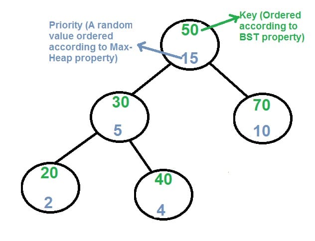
Priorities allow to uniquely specify the tree that will be constructed (of course, it does not depend on the order in which values are added), which can be proved using the corresponding theorem.
Obviously, if you choose the priorities randomly, you will get non-degenerate trees on average, which will ensure $O(\log{N})$ complexity for the main operations.
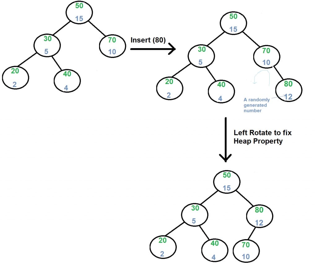
Insert: (e.g. x)
- Create new node with key equals to $x$ and value equals to a
randomvalue. - Perform standard BST insert.
- Use rotations to make sure that inserted node’s priority follows
max heap property.
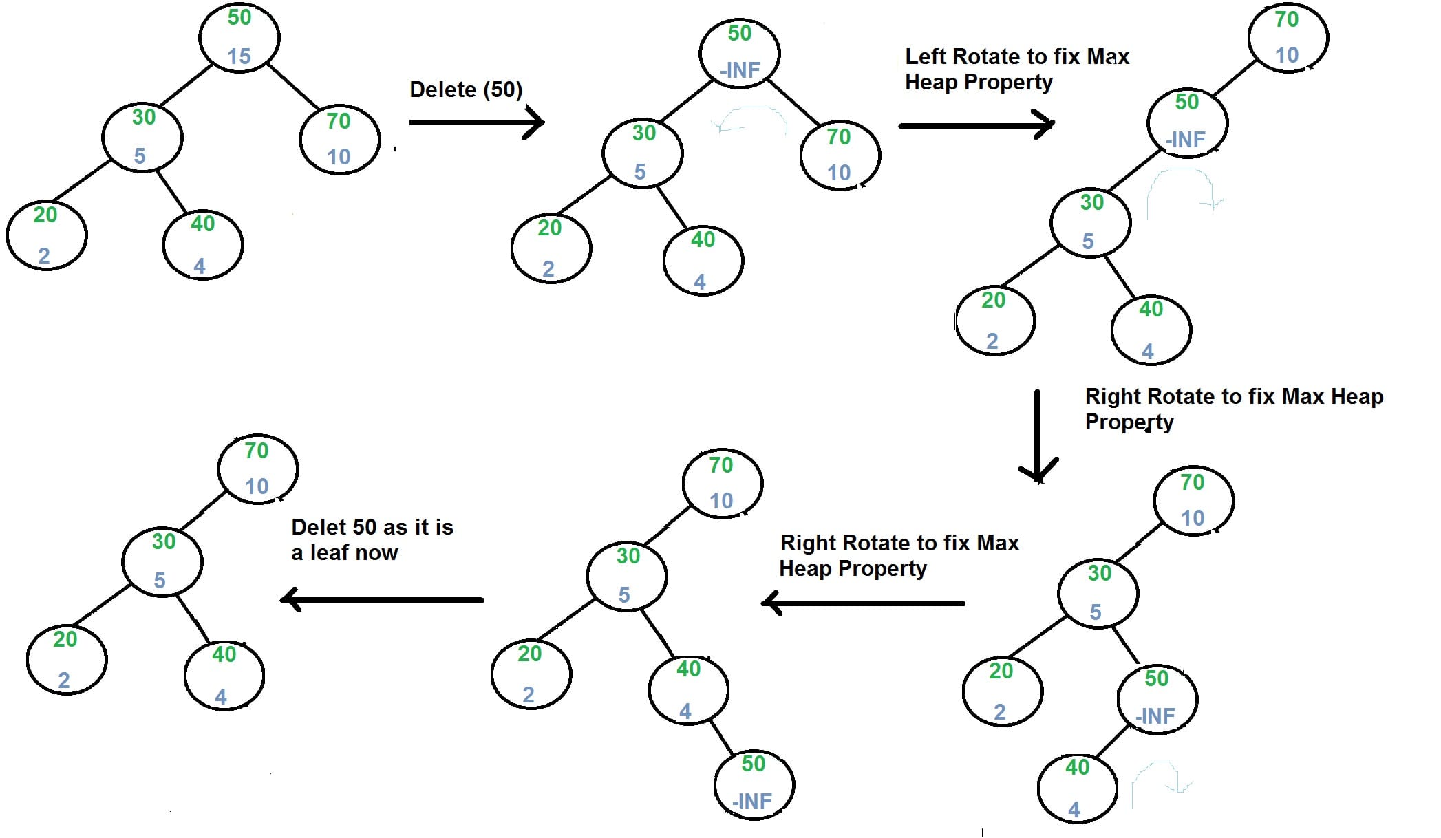
Delete: (e.g. x)
- If node to be deleted is a leaf, delete it.
- Else replace node’s priority with
minus infinite(-INF), and do appropriate rotations to bring the node down to a leaf.
Handle Duplicate Keys
A simple solution is to allow same keys on right side (also left side).
1 | 12 |
- Height may increase very fast.
A better solution is to augment every tree node to store count together with regular fields like key, left and right pointers.
1 | 12(3) |
- Height of tree is small irrespective of number of duplicates.
- Search, Insert, and Delete become easier to do. We can use same algorithms with small modification.