CS 61B | Part 3 | Asymptotic, Disjoint Set (Dynamic Connectivity)

Efficient Programming

Efficiency comes in two flavors:

• Programming cost (development)
• Execution cost (time and memory)

Terminology

Module: A set of methods that work together as a whole to perform some task or set of related tasks.

Encapsulated: A module is said to be encapsulated if its implementation is completely hidden, and it can be accessed only through a documented interface.

API: An API (Application Programming Interface) of an ADT is the list of constructors and methods (public) and a short description of each.

ADT: ADT (Abstract Data Type) is a high-level type that is defined by its behaviors, not their implementations.

• Deque in Proj1 is an ADT that had certain behaviors (addFirst, addLast, etc.). But, the data structures we actually used to implement it were ArrayDeque and LinkedListDeque.

• Some ADTs are actually special cases of other ADTs. For example, Stack and Queue are just Lists that have even more specific behaviors.

Extension & Delegation

1. Extension (Implementation Inheritance)

Borrow the methods from LinkedList<Item> and use them as its own.

public class ExtensionStack<Item> extends LinkedList<Item> {
  public void push(Item x) {
    add(x);
  }
}

2. Delegation (Abstraction)

Create a Linked List object and call its methods.

public class DelegationStack<Item> {
  private LinkedList<Item> L = new LinkedList<Item>();
  public void push(Item x) {
    L.add(x);
  }
}

3. Adapter (Assignable)

Similar to delegation, but it can use any class that implements the List interface (Linked List, ArrayList, etc.)

public class StackAdapter<Item> {
  private List L;
  public StackAdapter(List<Item> worker) {
    L = worker;
  }
  public void push(Item x) {
    L.add(x);
  }
}

Extension vs. Delegation: Right now it may seem that Extension and Delegation are pretty much interchangeable; however, there are some important differences that must be remembered when using them:

• Extension tends to be used when you know what is going on in the parent class.

  • In other words, you know how the methods are implemented.
  • Additionally, with extension, you are basically saying that the class you are extending from acts similarly to the one that is doing the extending.

• Delegation is when you do not want to consider your current class to be a version of the class that you are pulling the method from. It is independent (interface inheritance).

Idea of “View”

Views: An alternative representation of an existed object. Views essentially limit the access that the user has to the underlying object. However, changes done through the views will affect the actual object.

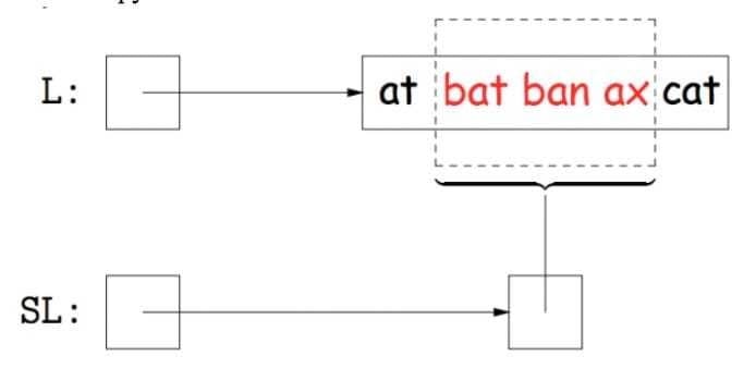
Issue: How do you return an actual List but still have it affect another List? Access methods

/** Assume in an Outer Class (MyList) */
List<Item> subList(int start, int end) {
  return new this.SubList(start, end); // Constructor
}

/** Inner Class */
private class SubList extends AbstractList<Item> {
  private int start, end;
  SubList(int start, int end) { ... }
  
  @Override
  public Item get(int k) {
    return AbstractList.this.get(start + k); // Gez
  }

  @Override
  public void add(int k, Item x) {
    AbstractList.this.add(start + k, x);
    end += 1;
  }
}

Usage:

List<Item> L = new MyList<>(); L.add(1); L.add(2); ...
List subL = L.subList(1, 3); /* subL is a SubList */
subL.get(1); /* equals to L.get(2) */
/* But we don't need to know its type is SubList */

An observation that should be made is that getting the k-th item from our subList is the same as getting the k-th item from our original list with an offset equal to our start index. Since we are using a get method of our outer class (the most parent one) we change our original list.

Similarly, adding an element to our subList is the same as adding an element to our original list with an offset equal to the start index of the subList.

The Takeaway

APIs are pretty hard to design; however, having a coherent design philosophy can make your code much cleaner and easier to deal with.

Implementation Inheritance (extension) is tempting to use frequently, but it has problems and should be used sparingly, only when you are certain about attributes of your classes (both those being extended and doing the extending).

Asymptotics

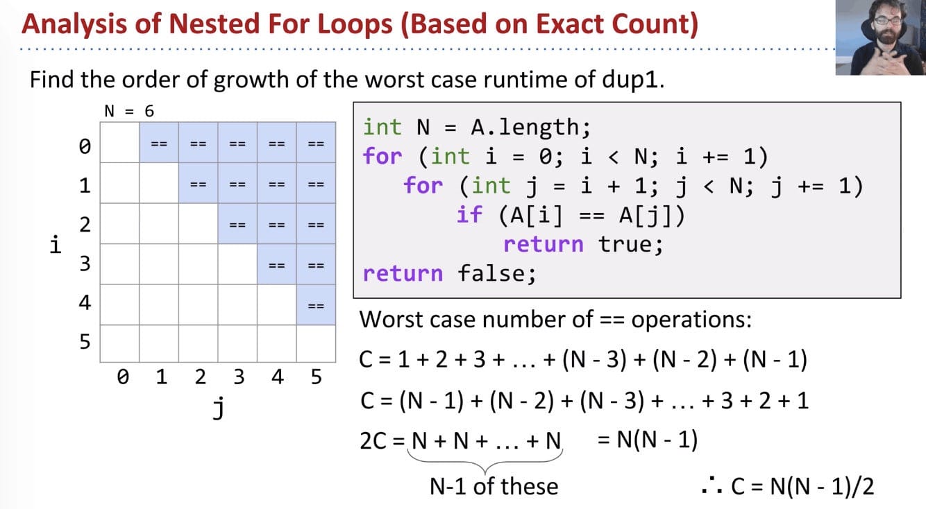
Counting

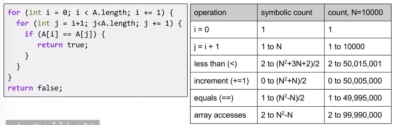
The problem is to check if there is a duplicate in the array.

Technique 2B: Count possible operations in terms of input array size $N$.

• Good: Machine independent. Input dependence captured in model. Tells you how algorithm scales.
• Bad: Even more tedious to compute. Doesn’t tell you actual time.

Comparison:

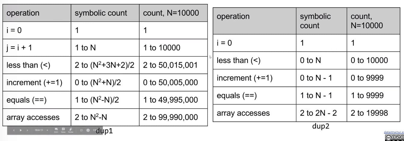
Which one is better? Three answers:

• An answer: It takes fewer operations to accomplish the same goal.
• Better answer: Algorithm scales better in the worst case $\frac{(N^2 + 3N + 2)}{2}$ vs. $N$.
• Even better answer: Parabolas $N^2$ grow faster than lines $N$.
  • Note: This is the same idea as our “better” answer, but it provides a more general geometric intuition.

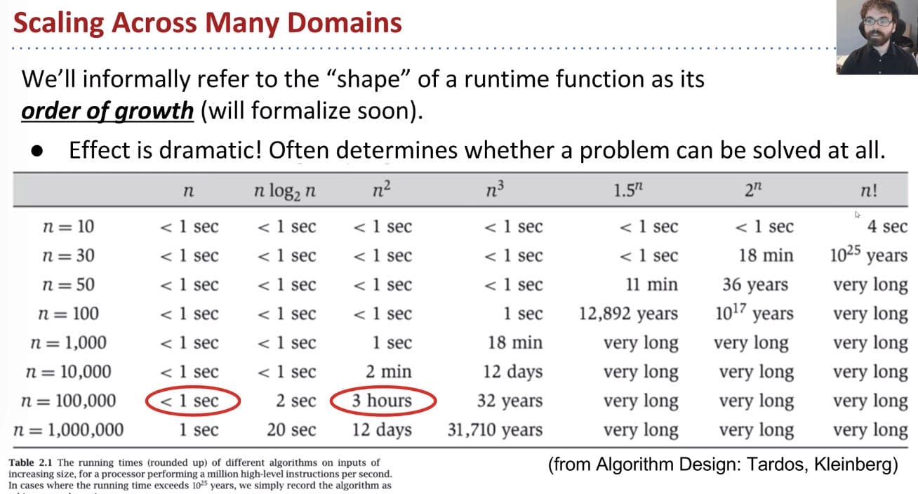
Simplification

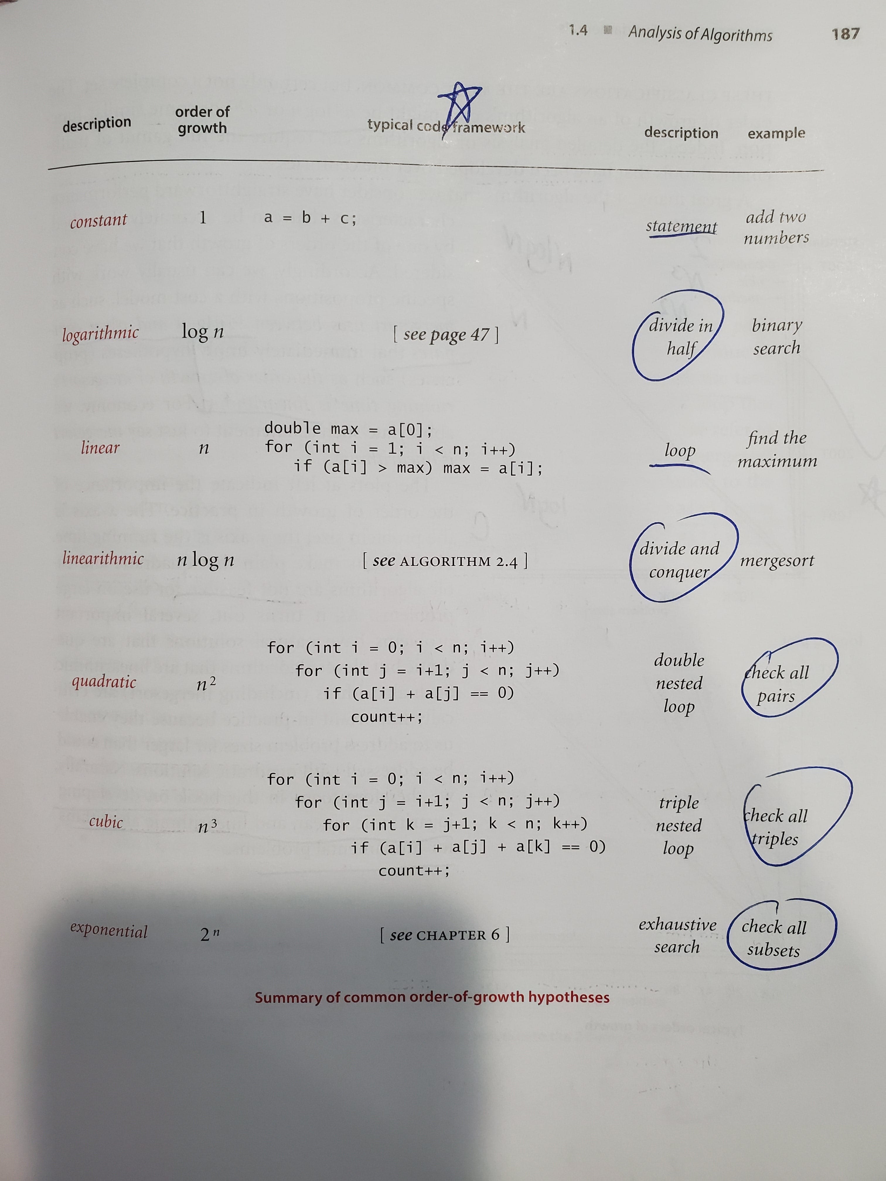
Convert the table into worst case o.o.g. (order of growth):

• Simplification 1: Consider only the Worst Case

  When comparing algorithms, we often only care about the worst case (though we’ll see some exceptions later in this course, like Quicksort?).

  • $N$ [linear]
  • $N^2$ [quadratic]
  • $N^3$ [cubic]
  • $N^6$ [sextic]

  Example: $\alpha (100 N^2 + 3N)+\beta (2 N^3 + 1) + 5000\gamma$

  For very large $N$, the $2\beta N^3$ term is much larger than the others.

• Simplification 2: Restrict Attention to One Operation

  Pick some representative operation to act as a proxy for overall runtime. The operation we choose can be called the cost model.

  for (int i = 0; i < A.length; ++i) {
    for (int j = i + 1; j < A.length; ++j) {
      if (A[i] == A[j]) {
        return true;
      }
    }
  }
  return false;

  • Good choice: increment, or < or ==, or array accesses.
  • Bad choice: assignment of j = i + 1, or i = 0 (since they execute only once).

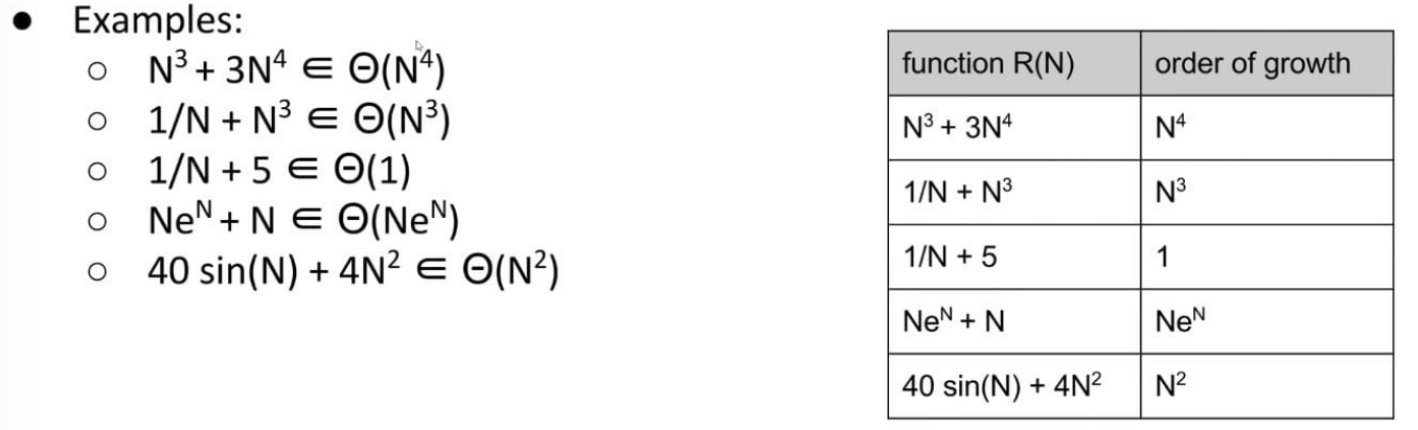
• Simplification 3: Eliminate Low Order Terms

  We can use tilde notation $\sim$ and ignore lower order terms.

• Simplification 4: Eliminate Multiplicative Constants

  Ignore multiplicative constants.

  Why? No real meaning! Remember that by choosing a single representative operation, we already “threw away” some information.

Summary:

1. Only consider the worst case.
2. Pick a representative operation (aka: cost model).
3. Ignore lower order terms
4. Ignore multiplicative constants

However, rather than building the entire table (it means counting table), we can instead:

1. Choose our cost model (representative operation we want to count).
2. Figure out the order of growth for the count of our representative operation by either:

• Making an exact count, and discarding unnecessary pieces.
• Using intuition / inspection to determine orders of growth.
  • Comes with practice!

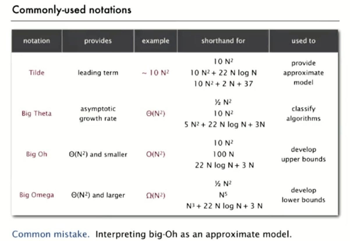
Big-Theta Notation

We only care about the o.o.g. of $R(N)$.

Given a piece of code, we can express its runtime as a function $R(N)$. Rather than finding $R(N)$ exactly, we instead usually only care about the order of growth of $R(N)$.

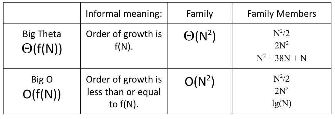
Big Theta $\Theta$ is exactly equivalent to order of growth. Suppose we have a function $R(N)$ with order of growth $f(N)$:

$$R(N) \in \Theta(f(N))$$

Big-Theta’s Formal Definition:

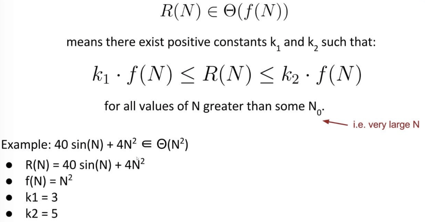
In other words, $R(N)$ is both upper and lower bounded by $\Theta(f(N))$.

Using Big-Theta doesn’t change anything about runtime analysis (no need to find $k_1$ or $k_2$ or anything like that).

The only difference is that we use $\Theta$ symbol anywhere we would have said “order of growth”, showing that we are considering the scale.

In summary, the approach is as follows:

• Choose a representative operation, and let $C(N)$ be the count of how many times that the operation occurs as a function of $N$.
• Determine order of growth $f(N)$ for $C(N)$, i.e. $C(N) \in \Theta(f(N))$.
  • Often (but not always) we consider the worst case count.
• If each operation takes constant time, then we say our runtime is $R(N) \in \Theta(f(N))$.

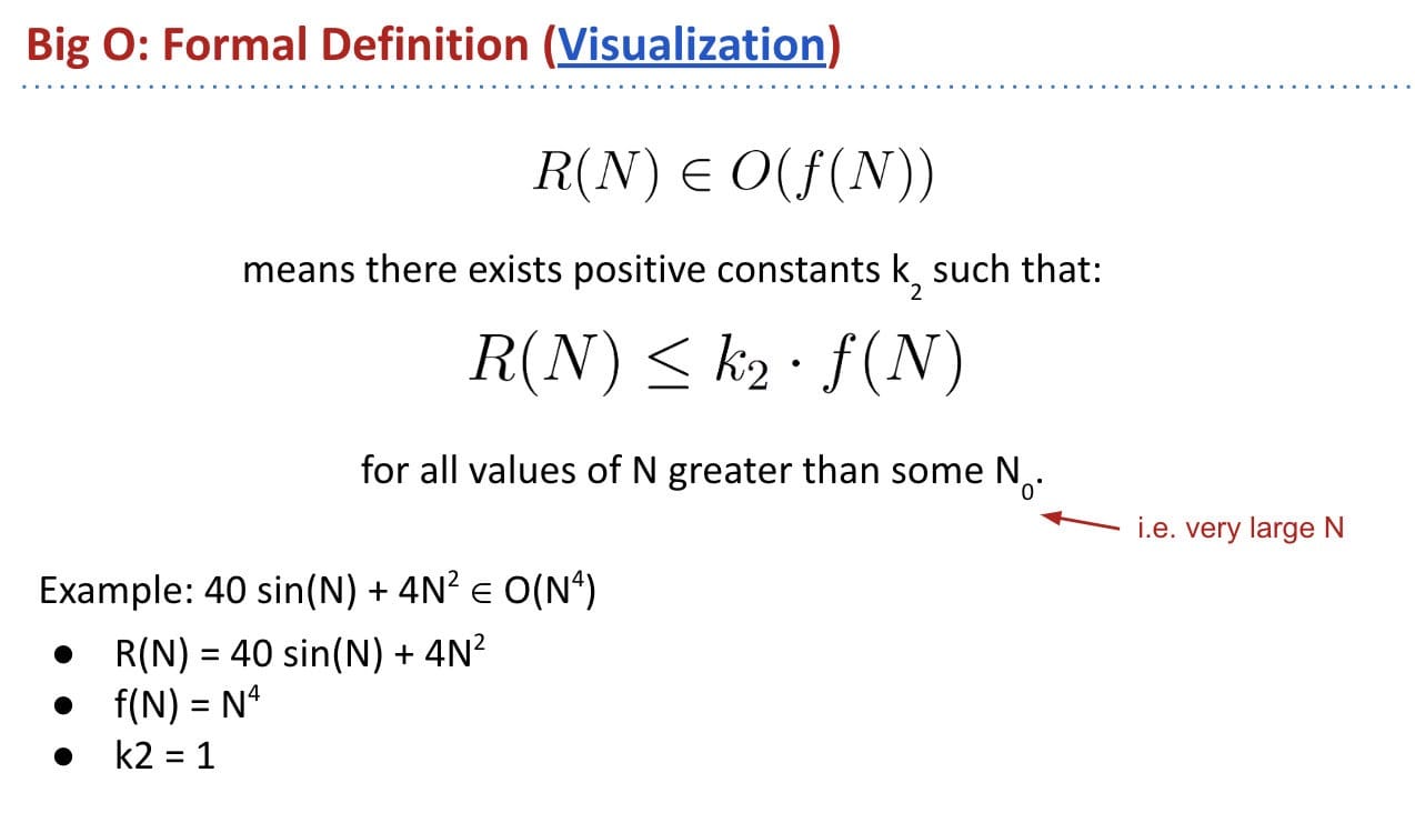
Big-O Notation

We use Big Theta to describe the order of growth of a function, or the rate of growth of the runtime of a piece of code.

For example, binary search on $N$ items has worst case runtime of $\Theta(log N)$.

Whereas Big Theta can informally be thought of as something like equals, Big O can be thought of as less than or equal.

In other words, $R(N)$ is only upper bounded by $f(N)$.

Comparison:

$N$ should be large enough:

Suppose we have a function bleepBlorp, and its runtime $R(N)$ has order of growth $\Theta(N^2)$. For large $N$, if we run bleepBlorp on an input of size $N$, and an input size $10N$, we will have to wait roughly 100 times as long for the larger input.

• True. It is the nature of quadratics.

If we run bleepBlorp on an input of size 1000, and an input of size 10000, we will have to wait roughly 100 times as long for the larger input.

• False. 1000 may not be a large enough $N$ to exhibit quadratic behavior.

Big-Theta vs. Big-O

Dependency On Input:

Consider a trick question:

// same version
public boolean dup4(int[] a) {
  int N = a.length;
  for (int i = 0; i < N; ++i) {
    for (int j = i + 1; j < N; ++j) {
      if (a[i] == a[j]) {
        return true;
      }
    }
  }
  return false;
}

Let $R(N)$ be the runtime of the code below as a function of $N$. What is the order of growth of $R(N)$?

1. $\Theta(1)$
2. $\Theta(N)$
3. $\Theta(N^2)$
4. Something else (depends on the input) (X)

Analysis:

• The best case runtime: $\Theta(1)$
• The worst case runtime: $\Theta(N^2)$

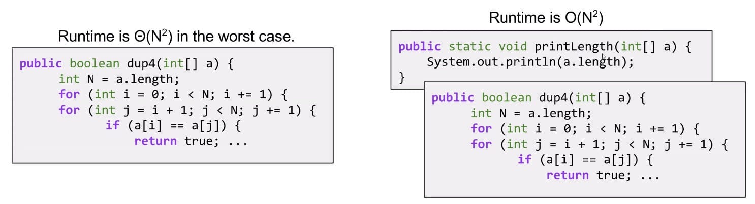
In this case, we can just use Big-O to avoid qualifying our statement at all, i.e. $O(N^2)$ includes a sense that the runtime could possibly be $\Theta(1)$.

The Limitations of Big Theta:

Big-Theta expresses exact order of growth for runtime in terms of $N$. If runtime depends on more factors than just $N$, we may need different Big Theta for every interesting condition.

Big-O Is Less Informative:

Which statement gives you more specific information about the runtime of a piece of code?

1. The worst case runtime is $\Theta(N^2)$. (X)
2. The runtime is $O(N^2)$. (it exhibits too much)

Example:

Common Usage:

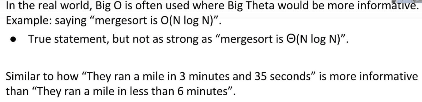
Note: Despite lower precision, Big-O is used way more often in conversation. Although it does not mean “worst case”, it is often abused to mean this and used as such.

However, Big-O is still a useful idea:

• Allows us to make simple blanket statements without case qualifications.
  • E.g. we can just say “binary search is $O(\log{N})$” instead of “binary search is $\Theta(\log{N})$ in the worst case”.
• Sometimes don’t know the exact runtime, so use $O$ to give an upper bound.
  • Example: Runtime for finding shortest route that goes to all world cities is $O(2^N)^*$. There might be a faster way, but nobody knows one yet.
• Easier to write proofs for Big-O than Big-Theta.

Big-Omega Notation

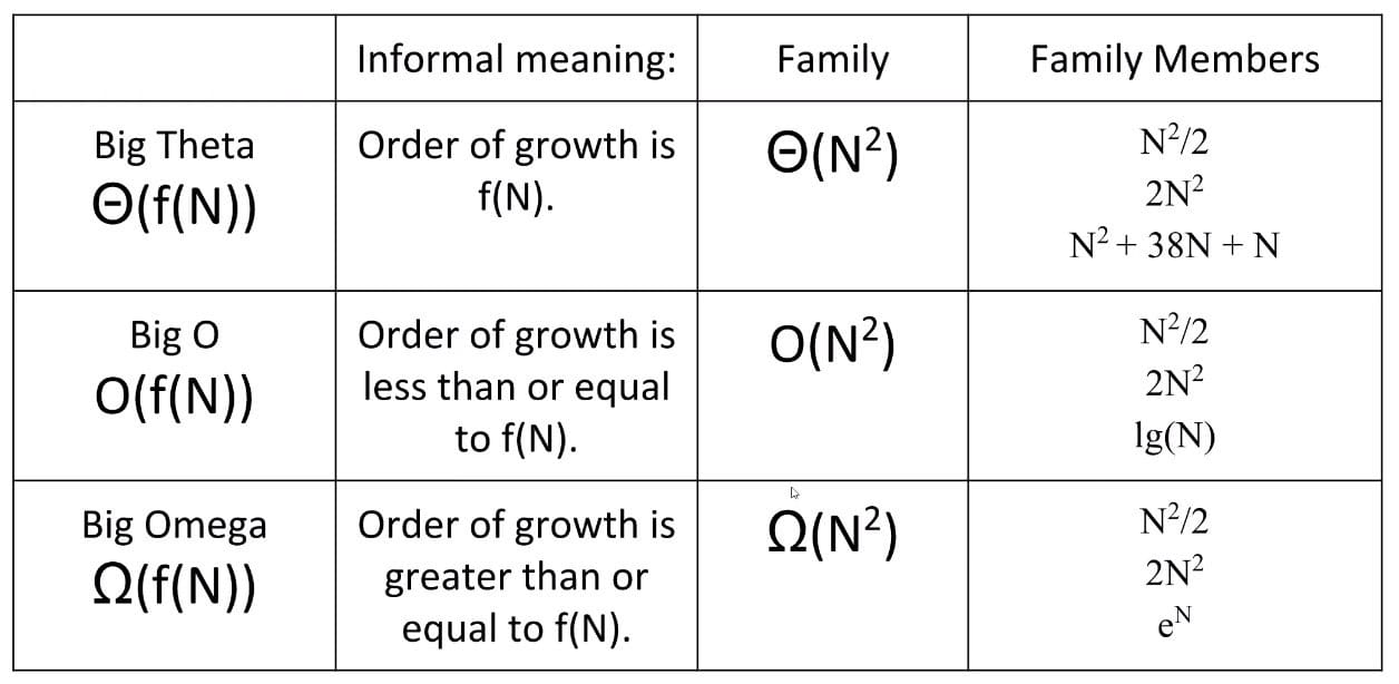
Two common uses for Big-Omega:

• Very careful proofs of Big-Theta runtime.
  • If $R(N) = O(f(N))$ and $R(N) = \Omega(f(N))$, then $R(N) = \Theta(f(N))$.
  • Sometimes it’s easier to show $O$ and $\Omega$ separately.
• Provide lower bounds for the hardness of a problem (the best case).
  • Example: The time to find whether an array has duplicates is $\Omega(N)$ in the worst case since we have to actually look at every item.

Note: Big-Omega does not mean best case.

Amortized Analysis

It provides a way to prove the average cost of operations.

Grigometh’s Hay

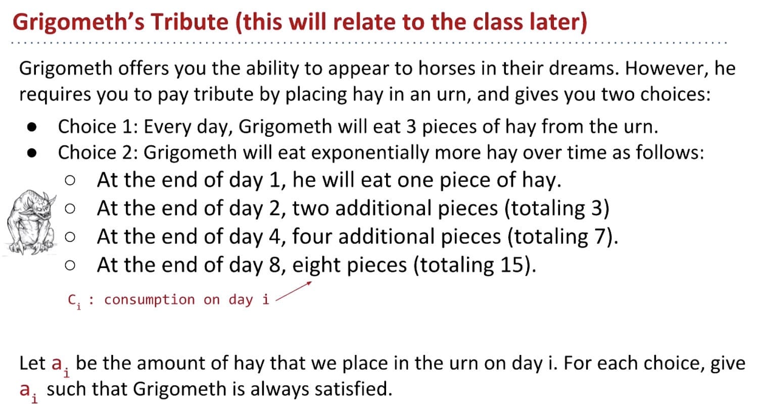
Note: Just like the growth of a binary tree by levels.

Punchline: Grigometh’s consumption per day is effectively constant.

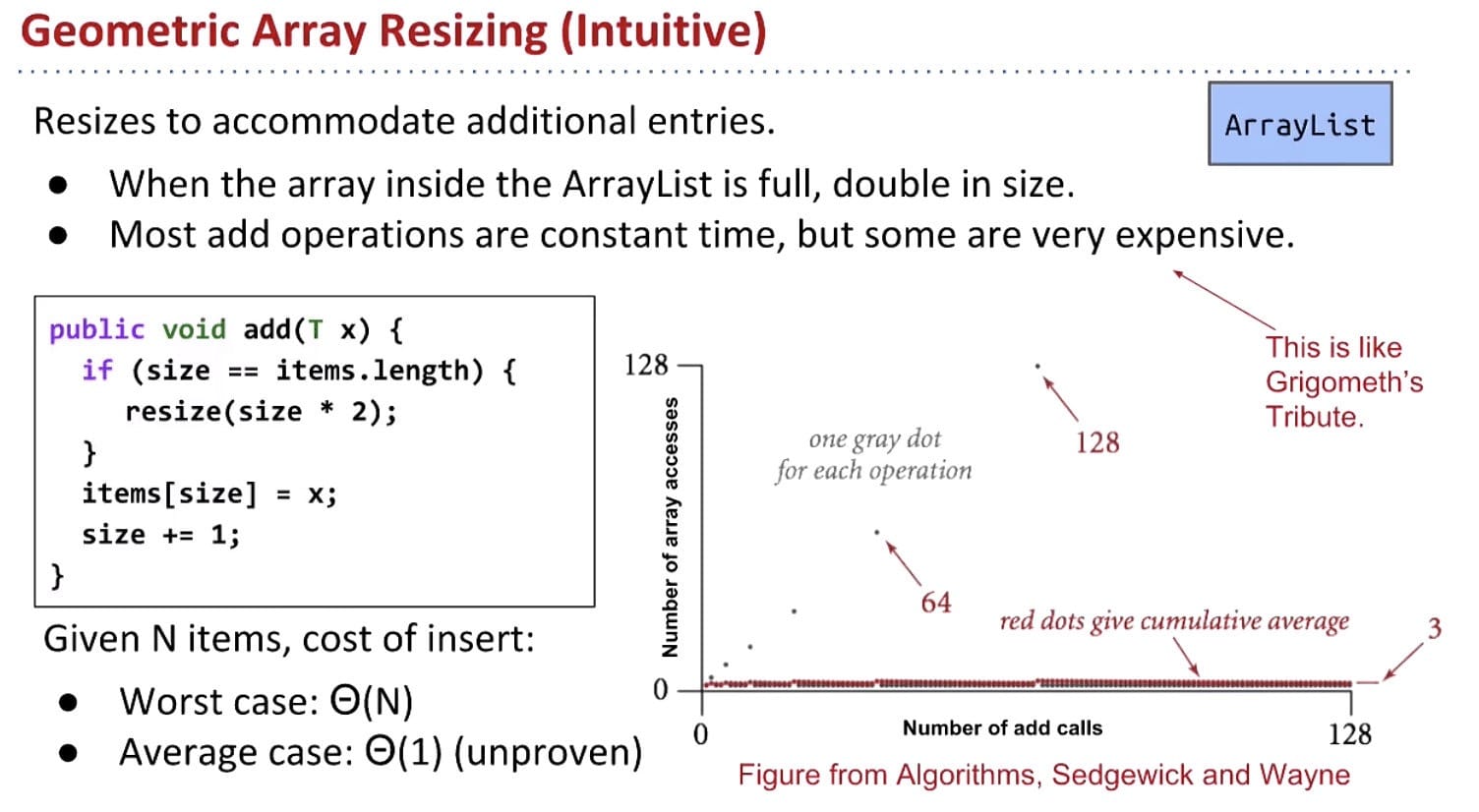
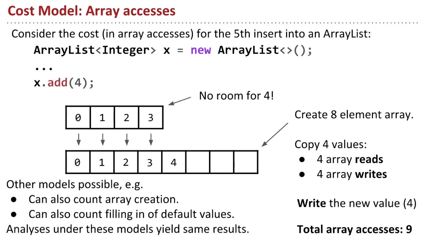
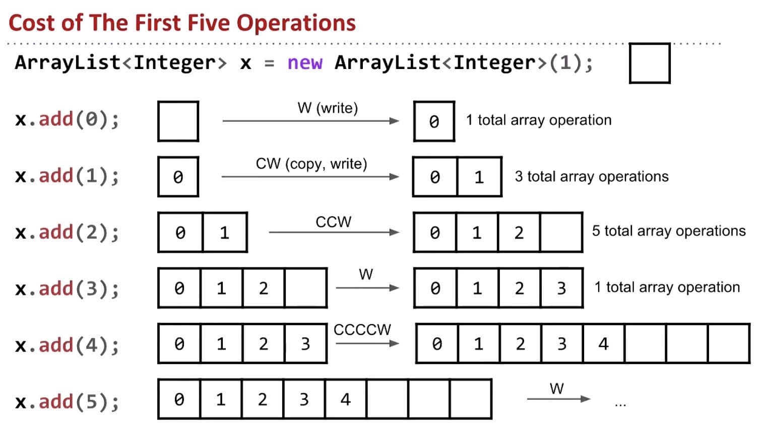
Geometric Resizing

It turns out, Grigometh’s hay dilemma is very similar to AList resizing.

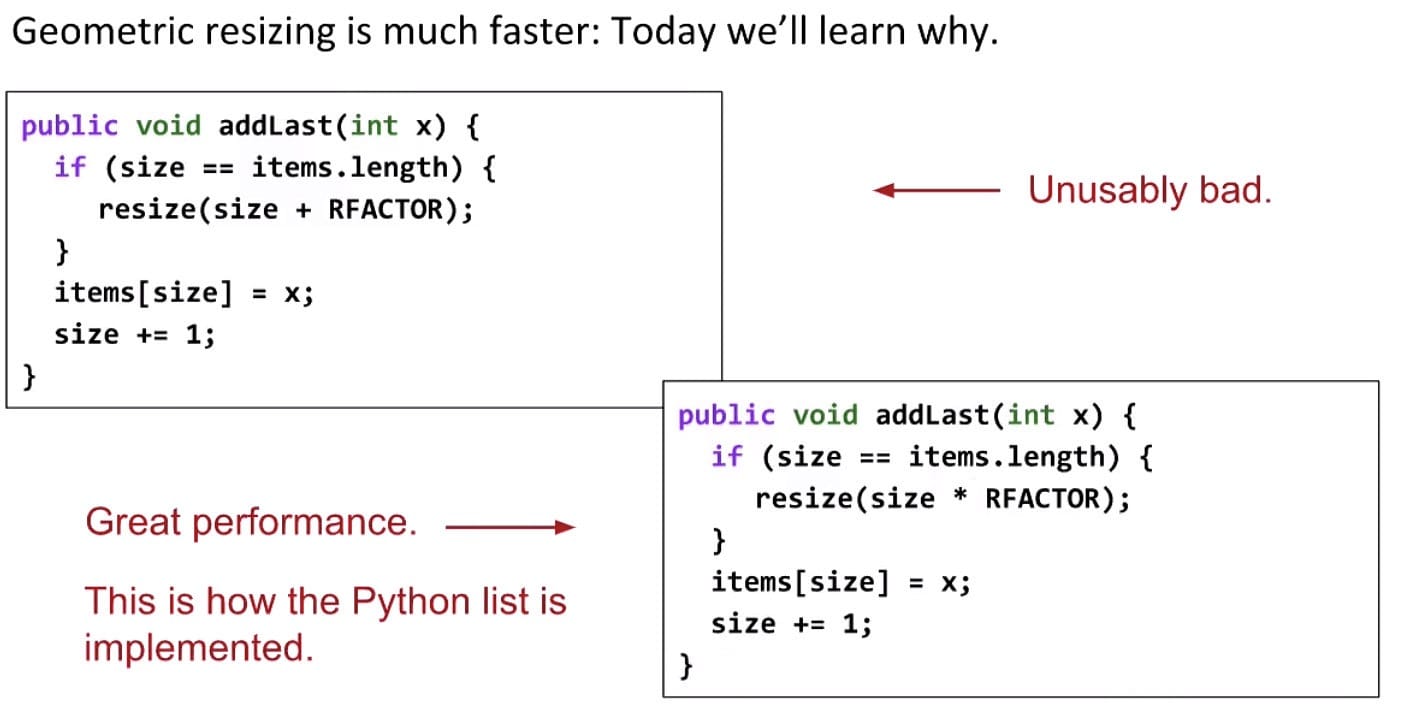
As for the second implementation, most add operations take $\Theta(1)$ time, but some are very expensive, and linear to the current size. However, if we average out the cost of expensive adds with resize, overall the adds that are cheap. And it turns out that on average, the runtime of add is $\Theta(1)$.

A more rigorous examination of amortized analysis is done here, in three steps:

• Pick a cost model (like in regular runtime analysis).
• Compute the average cost of the i-th operation.
• Show that this average (amortized) cost is bounded by a constant.

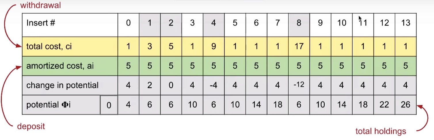
Even though some elements cost linear time $\Theta(N)$, average cost of each insert is $\Theta(1)$.

• Amortized total cost seems to be about $(44 / 14) = 3.14$ accesses / item.

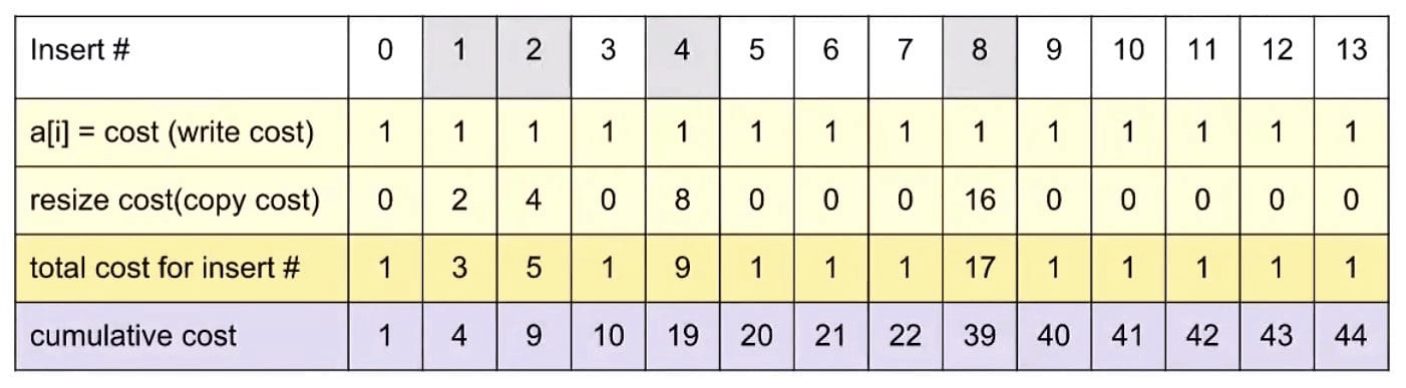
Note: For the first 8 adds, the average cost is 39/8 = 4.875 per add. It seems like it might be bounded by 5. But just by looking at the first 13 adds, we cannot be completely sure.

How do we prove it?

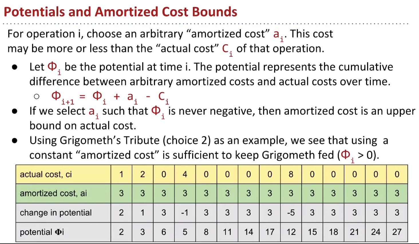
The Idea of Potential

We’ll now introduce the idea of potential to aid us in solving this amortization mystery.

Idea: Select an amortized cost $a_i$ such that potential $\Phi_i$ is never negative.

Now back to ArrayList resizing

For ArrayList, the goal: $a_i \in \Theta(1)$ and $\Phi_i \geq 0$ for all $i$.

Finally, we’ve shown that ArrayList add operations are indeed amortized constant time. Geometric resizing (multiplying by the RFACTOR) leads to good list performance.

Extra Notes (algs4)

An algorithm must be seen to be believed. – Donald Knuth

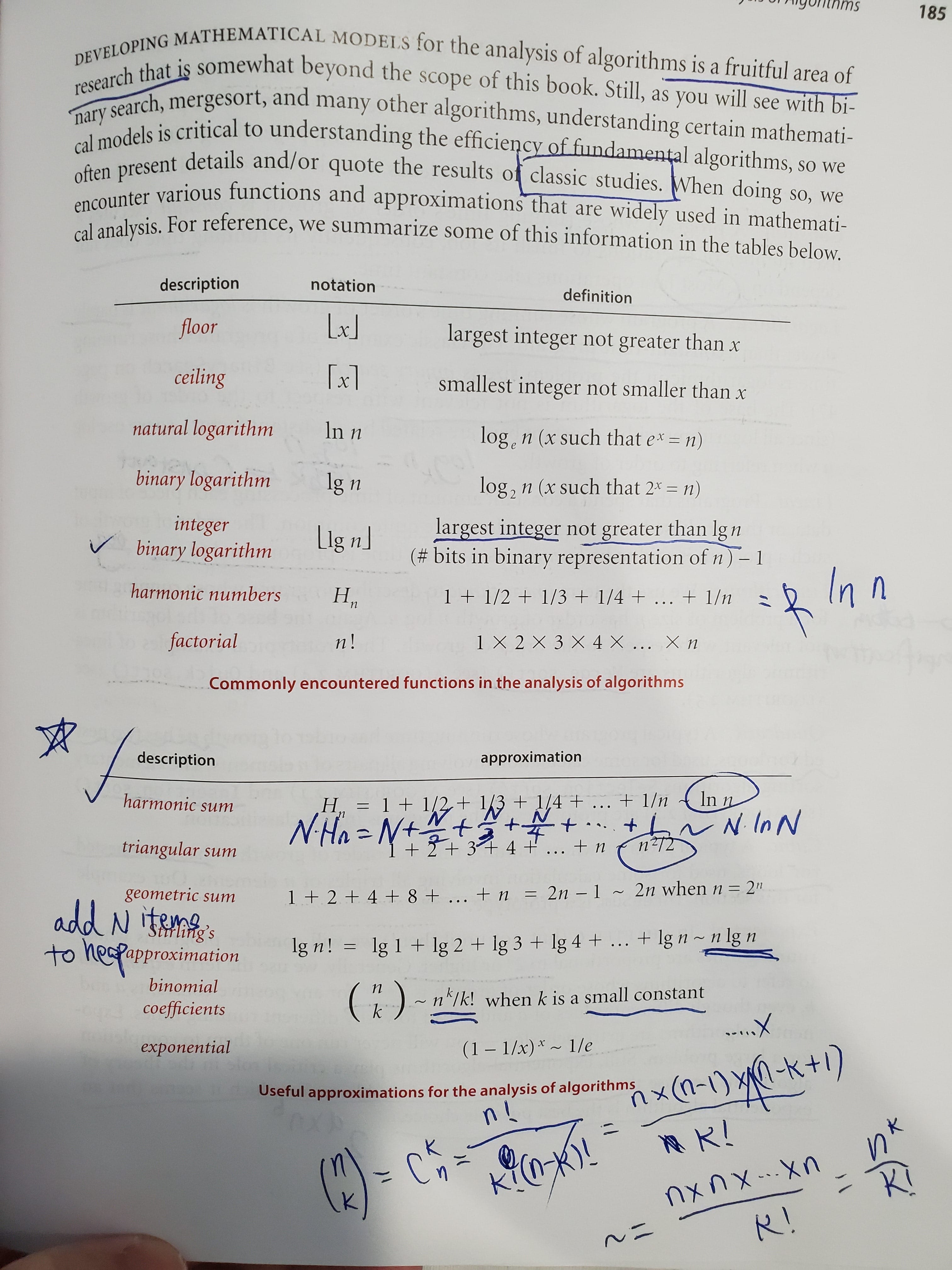
Log million, lg(1,000,000), is approximately 20.

$1 + \frac{1}{2} + \frac{1}{3} + … + \frac{1}{N} = \ln N$

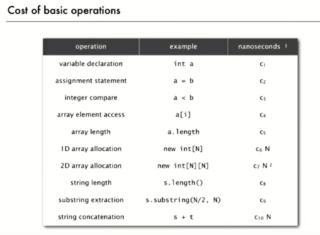
Note: Cost of substring extraction is constant.

61B Style:

The TA demonstrates a general model to solve this kind of problems.

Steps:

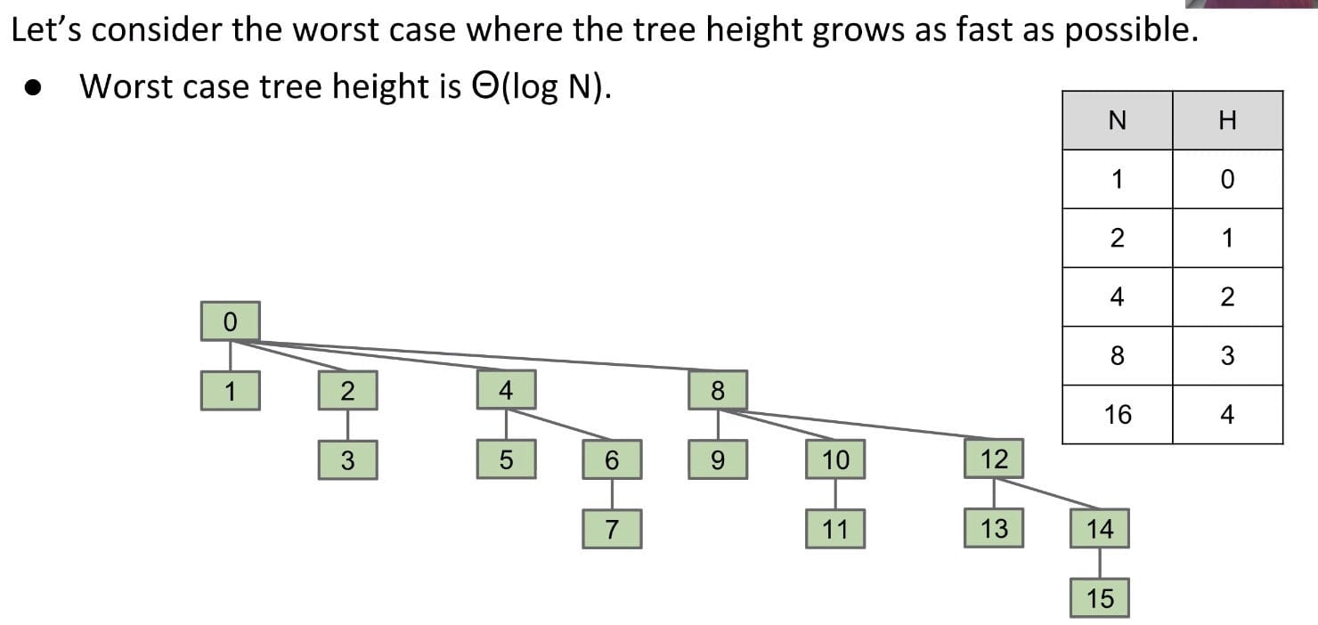
• Height of Tree (layers)
  • $h = \log N$
• Branching Factor (#node = #subproblem)
  • Note each time andslam() is called, it makes 1 recursive call on n/2
  • #node per layer is 1
• Amount of Work each node / layer does ($f(N) = D(N) + C(N)$)
  • Sometimes it includes println, merging and combining time, etc.

Note: In Discussion 7, Spring 2019.

Ex (In-Class Practice)

Ex 1 (i *= 2)

Problem:

Note: We drop some information for easily computation. Remember to use tilde notation ~.

Solution:

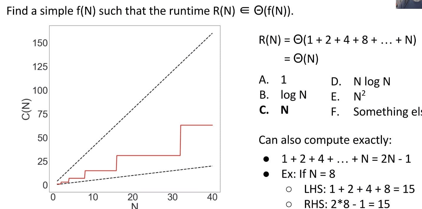
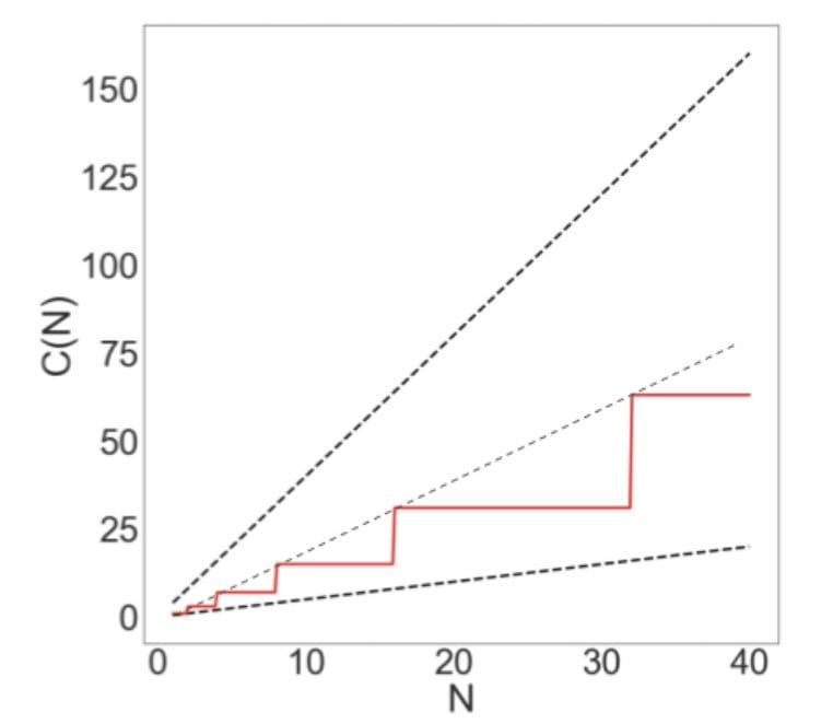
Since the red line is bounded by two linear lines ($N$ and $4N$), the runtime must also be linear!

If we compute the “exact” count, we have a stricter bound $2N - 1$:

$$
\begin{aligned}
C(N) &= 2^0 + 2^1 + 2^2 + \ldots + 2^{lgN}\
&= 2^{(lgN + 1)} - 1\
&= 2^{(lgN + lg2)} - 1\
&= 2^{lg2N} - 1\
&= 2N - 1\
\end{aligned}
$$

So we can draw a new line in the graph $C(N) = 2N - 1$:

It would be super convenient if all nested for loops were $N^2$. However, they’re not.

Caveats For Runtime Analysis:

• There is no magic shortcut for these problems.
• Runtime analysis often requires careful thought.
  • In programming, one little tiny statement in the middle of the code can cause the runtime to be completely different.
  • Therefore, we can’t always assume that the runtime of a statement takes constant time.
• In this class, there are basically two sums you need to know:
  • Sum of First Natural Numbers: $1 + 2 + 3 + … + Q = \frac{Q(Q+1)}{2} = \Theta(Q^2)$
  • Sum of First Powers of Two: $1 + 2 + 4 + 8 + … + Q = 2Q - 1 = \Theta(Q)$
• Strategies:
  • Find exact sum
  • Write out examples
  • Draw graphs

Ex 2 (j *= 2)

Consider the variant of the previous example:

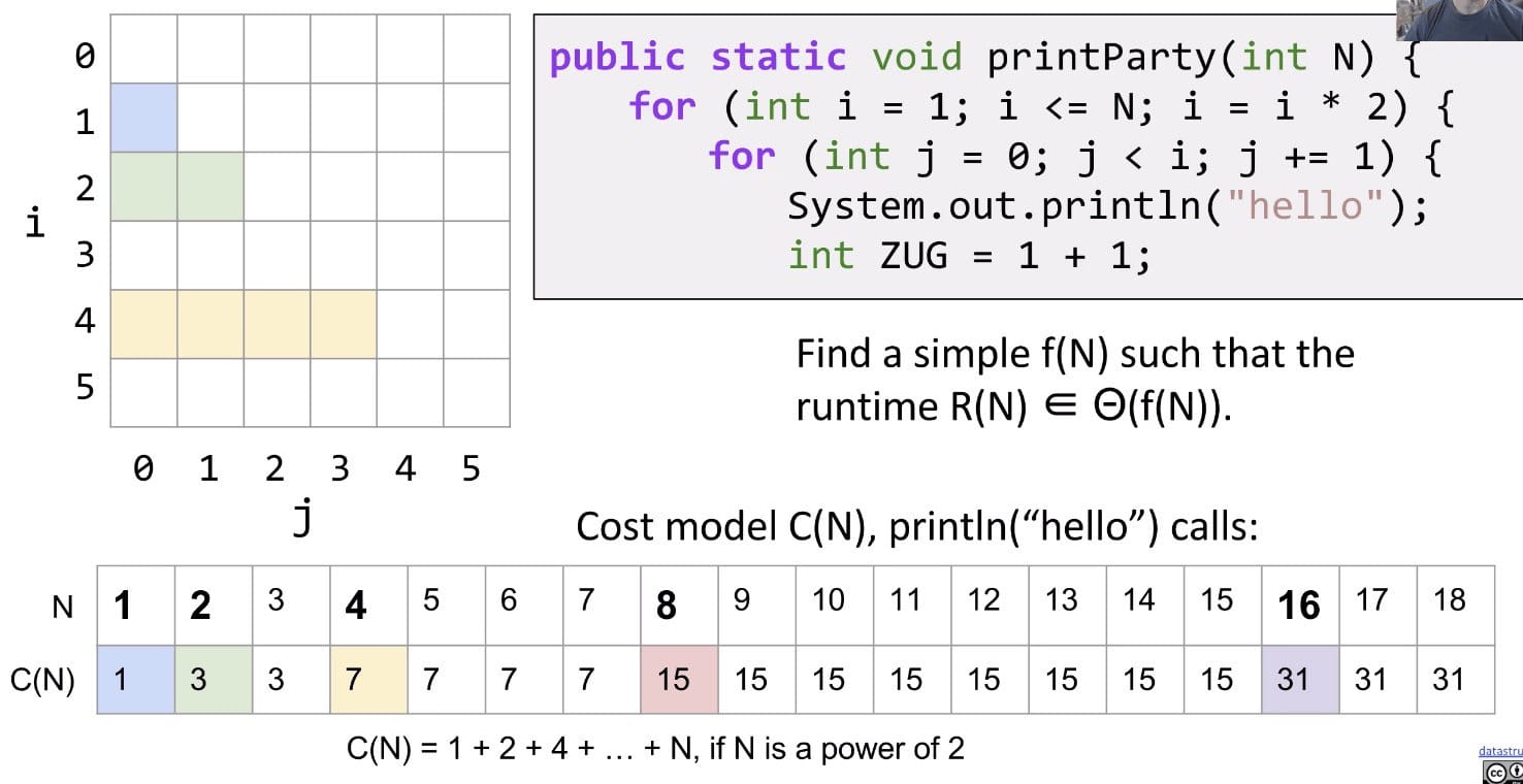
public static void printParty(int N) {
  for (int i = 0; i < N; i += 1) { // N times
    for (int j = 1; j < N; j *= 2) { // 1 ~ lgN
      System.out.println("Show me the code!");
    }
  }
}

Cost model: println
Analysis:

• The outer loop will execute ~$N$ times. The inner loop grows very fast: Execute 0, 1, 2, 2, 3, 3, 4, …, 4, …, lgN times each.
• It is difficult to sum it up so we better look into its upper bound. Let each inner loop execute $\log{N}$ times, so we have runtime $O(N\log{N})$.

Ex 3 (Binary Search)

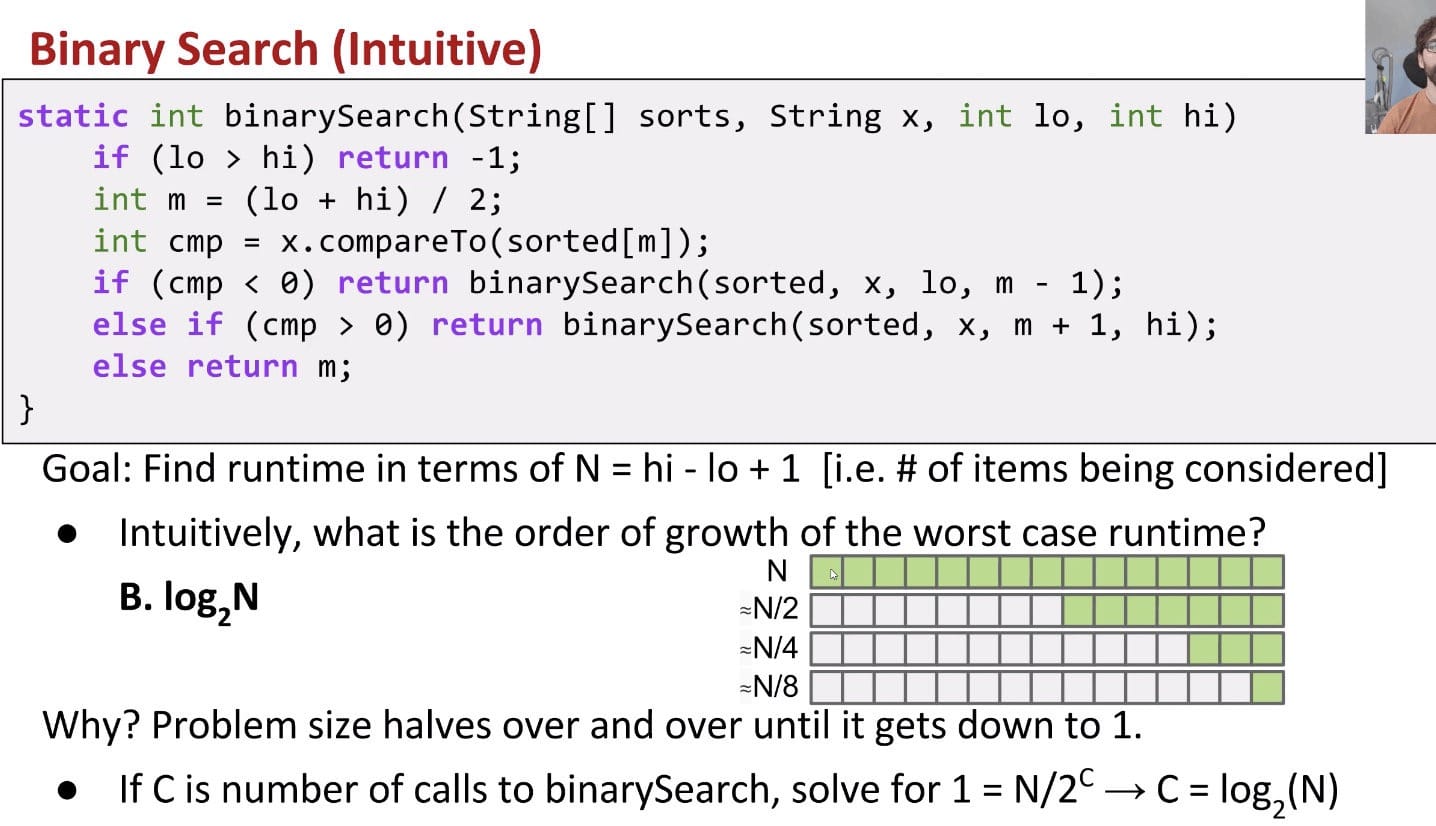
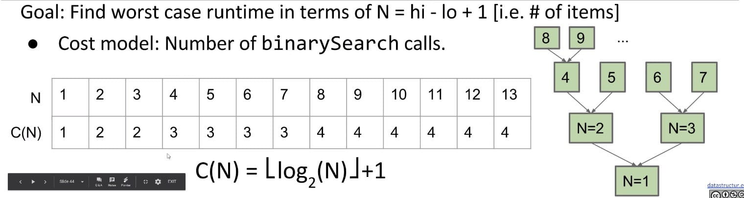
Note: Cost model could also be the comparison statement. The worst case runtime of Binary Tree is determine by the height of the tree.

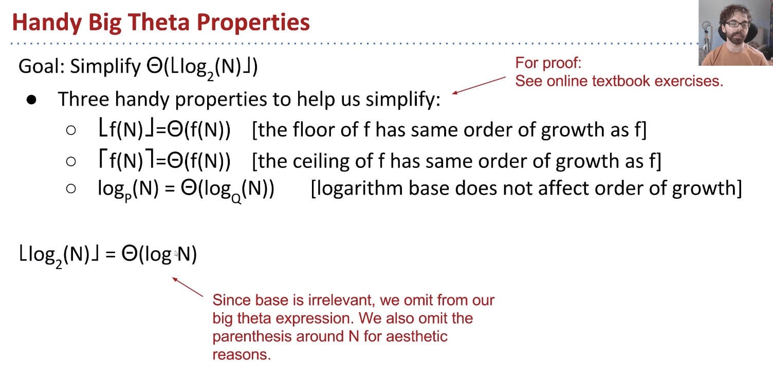
The last one essentially states that for logarithmic runtimes, the base of the logarithm doesn’t matter at all, because they are all equivalent in terms of Big-O (this can be seen by applying the logarithm change of base).

According to: $\log_b(a) = \frac{\log_x(a)}{\log_x(b)}$, we have: $\log_P(N) = \frac{\log_Q(N)}{\log_Q(P)}$.

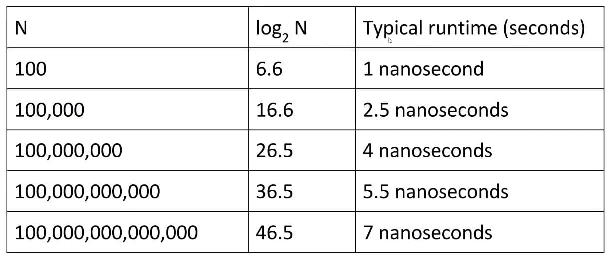
Log time is super good! In practice, logarithmic time algorithms have almost constant runtime. Even for incredibly huge datasets, practically equivalent to constant time.

Ex 4 (f(n-1) + f(n-1))

public static int f3(int n) {
  if (n <= 1)
    return 1;
  return f3(n - 1) + f3(n - 1);
}

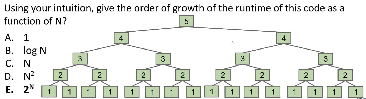
It’s the recursion tree on which we can guess the runtime.

Cost model: #calls to $f_3$.

Firstly, draw out the recursion tree to get an intuitive feeling or guess.

Secondly, write down number of operations at each level.

• 1st level: 1 x f(5)
• 2nd level: 2 x f(4)
• 3rd level: 4 x f(3)
• 4th level: 8 x f(2)
• …
• Nth level: 2^(N-1) x f(1)

Sum: According to sum of first powers of 2, O(2 x 2^(N-1) - 1) = O(2^N)

More Formal Version (CDQ):

It is a CDQ problem and the time complexity recurrence is as follows:

$$T(N) = 2T(N-1) + D(N) + C(N) = 2T(N-1)$$

But it could not be solved by the master method, since $b$ could not be expressed by a constant.

Ex 5 (Mergesort)

Selection sort:

• Find the smallest unfixed item, move it to the front, and ‘fix’ it.
• Sort the remaining unfixed items using selection sort.

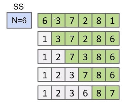
Given that runtime is quadratic, for N = 64, we might say the runtime for selection sort is 2,048 arbitrary units of time (AU).

• N = 6 => ~36 AUs
• N = 64 => ~2048 AUs (Shouldn’t it be 4096 ???)

Array Merging:

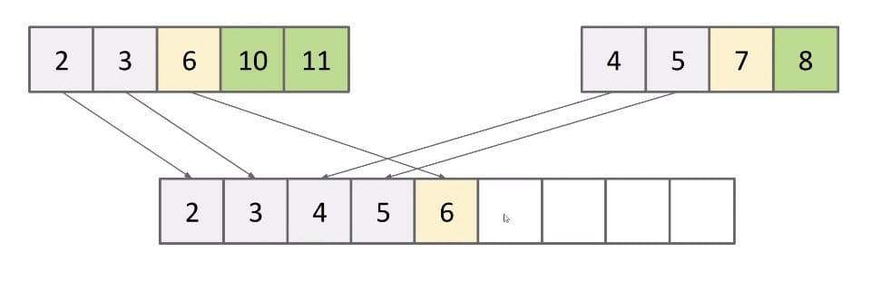
The runtime is $\Theta(N)$. Use array writes as cost model.

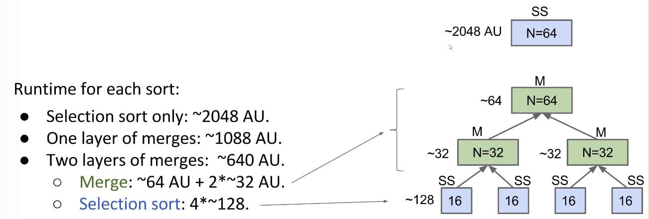
Improvement

Merging can give us an improvement over vanilla selection sort:

• Selection sort the left half: $\Theta(N^2)$
• Selection sort the right half: $\Theta(N^2)$
• Merge the results: $\Theta(N)$

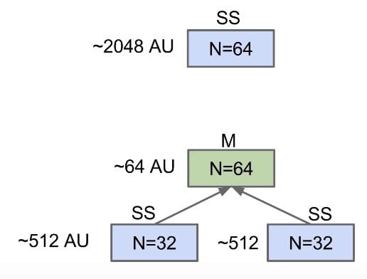
Still $\Theta(N^2)$, but faster since $N + 2 \times (\frac{N}{2})^2 < N^2$

And we can go on doing it:

Mergesort

Mergesort does merges all the way down (no selection sort):

1. If array is of size 1, return.
2. Mergesort the left half.
3. Mergesort the right half.
4. Merge the results: $\Theta(N)$

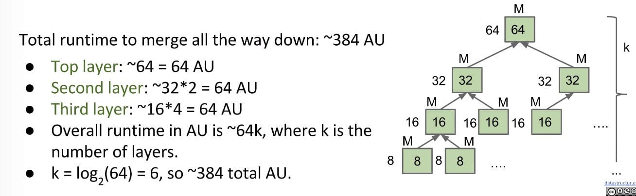
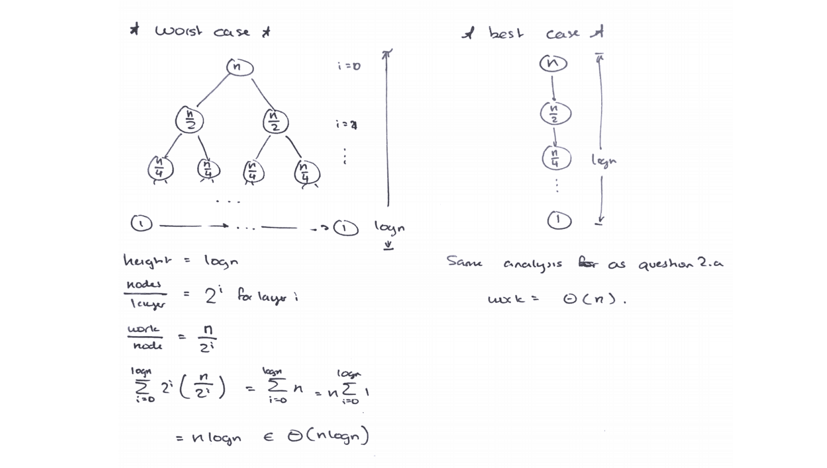
For an array of size $N$, what is the worst case runtime of Mergesort?

For $N$, there will be $\log(N)$ layers, and each layer contains $N$ AUs. So in total there are $N\log(N)$ AUs.

More Formally:

Mergesort is a classic CDQ problem and its runtime could be written as a recurrence form:

$$
\begin{aligned}
f(N) &= D(N) + C(N) = \Theta(N)\
T(N) &= 2T(N/2) + f(N) = 2T(N/2) + \Theta(N)\
\end{aligned}
$$

According to the master method, the runtime of this case is $O(N\log{N})$.

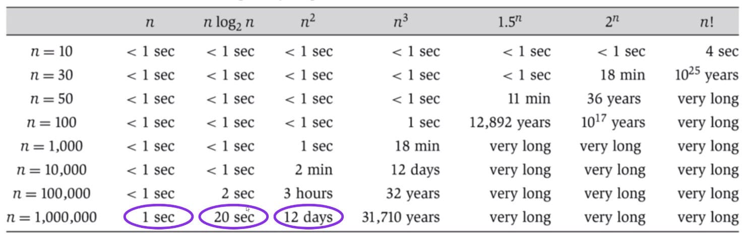
How good the linearithmic runtime is?

$N\log N$ is basically as good as $N$, and is vastly better than $N^2$.

Going from $N\log N$ to $N$ is nice, but not a radical change, just like going from $\log{N}$ to $1$.

Ex (Discussion 7)

• Any exponential $k^n$ dominates any polynomial $n^k$
• Any polynomial dominates any logarithm

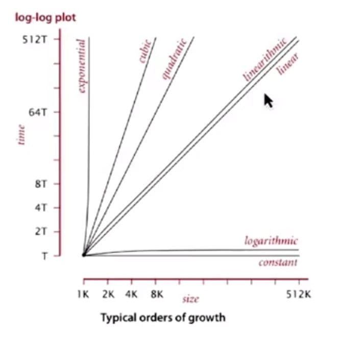
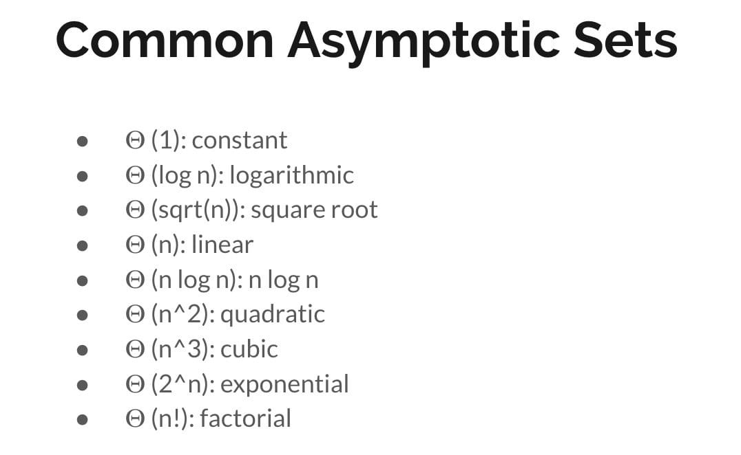
Increasing Order of Time Complexity:

$\Theta(1) < \Theta(\log{n}) < \Theta(n) < \Theta(n\log{n}) \sim \Theta(\log{n!}) < \Theta(n^2) < \Theta(n^2 \log{n}) < \Theta(n^3) < \Theta(2^n) < \Theta(n!) < \Theta(n^n)$

Ex 1 (ping)

int j = 0;
for (int i = N; i > 0; --i) {
  for (; j <= M; ++j) {
    if (ping(i, j) > 64) {
      break;
    }
  }
}

Here we need to choose 2 cost models: i > 0 and j <= M or if (). It’s very similar to the runtime analysis of graph problems, since the outer and inner loops are irrelevant.

Runtime: $O(N + M)$

Ex 2 (mystery)

public static boolean mystery(int[] array) {
  array = mrpoolsort(array); // NlogN
  int N = array.length;
  for (int i = 0; i < N; ++i) {
    boolean x = false;
    for (int j = 0; j < N; ++j) {
      if (i != j && array[i] == array[j]) {
        x = true;
      }
    }
    if (!x) { // if (x == false)
      return false;
    }
  }
  return true;
}

Worst: $\Theta(N \log{N} + N^2) = \Theta(N^2)$
Best: $\Theta(N \log N + N) = \Theta(N \log N)$ (when i = 0, survive during the first inner loop. x stays false)

Ex 3 (comeOn)

for (int i = 0; i < N; ++i) {
  for (int j = 1; j <= M; ) {
    if (comeOn()) {
      j += 1;
    } else {
      j *= 2;
    }
  }
}

Worst: $\Theta(NM)$, when comeOn() always returns true.
Best: $\Theta(N \log M)$, when comeOn() always returns false.

Ex 4 (findSum)

Note: the array is sorted!

/* Naive */
public static boolean findSum(int[] A, int x) {
  for (int i = 0; i < A.length; i++) { // N
    for (int j = 0; i < A.length; j++) { // N
      if (A[i] + A[j] == x) {
        return true;
      }
    }
  }
  return false;
}

Worst: $\Theta(N^2)$
Best: $\Theta(1)$, when i = 0 and j = 0 and A[i] + A[j] == x.

/* Optimized Version: Using two pointers */
public static boolean findSumFaster(int[] A, int x) {
  // 1 2 3 4 5 6 7
  // i           j  left: i   right: j
  int left = 0; int right = A.length - 1;
  while (left <= right) {
    if (A[left] + A[right] == x) {
      return true;
    } else if (A[left] + A[right] < x) {
      left += 1;
    } else {
      right -= 1;
    }
  }
  return false;
}

Worst: $\Theta(N)$
Best: $\Theta(1)$

Ex 5 (Union & Intersection)

Implementation of Union & Intersection of Two Arrays:

Union:

/* Union */
public static int[] union(int[] A, int[] B) {
  HashSet<Integer> set = new HashSet<>();
  for (int num : A) { // add to set
    set.add(num);
  }
  for (int num : B) {
    set.add(num);
  }
  int[] unionArray = new int[set.size()]; // to array
  int index = 0;
  for (int num : set) {
    unionArray[index] = num;
    index += 1;
  }
  return unionArray;
}

Intersection:

/* Intersection */
public static int[] intersection(int[] A, int[] B) {
  HashSet<Integer> setOfA = new HashSet<>();
  HashSet<Integer> intersectionSet = new HashSet<>();

  for (int num : A) {
    setOfA.add(num);
  }

  for (int num : B) {
    if (setOfA.contains(num)) {
      intersectionSet.add(num);
    }
  }

  int[] intersectionArray = new int[intersectionSet.size()]; // to array
  int index = 0;
  for (int num : intersectionSet) {
    intersectionArray[index] = num;
    index += 1;
  }
  return intersectionArray;
}

Ex (Guide)

Ex 1 (Memo Fibonacci)

Traditional Manner:

public int fib(int n) {
  if (n <= 1) return n;
  return fib(n - 1) + fib(n - 2);
}

$N$	0	1	2	3	4	5	6
$C(N)$	0	0	3	5	9	15	25

$C(N) = C(N - 1) + C(N - 2)$
$C(N) = (\frac{1 + \sqrt{5}}{2})^N + (\frac{1 - \sqrt{5}}{2})^N$
$T(N) = O((\frac{1 + \sqrt{5}}{2})^N + (\frac{1 - \sqrt{5}}{2})^N) = O((\frac{1 + \sqrt{5}}{2})^N) = O(1.6180^N)$

Reference: link

Faster Manner:

Assume that values is an array of size $n$. If a value in an int array is not initialized to a number, it is automatically set to 0.

// 0   1   2   3   4   5
// 0   0   0   0   0   0
// n-2 n-1 n
// Note: values's size should be n + 1 including 0 and 1~n
public void modified_fib(int n, int[] values) {
  if (n <= 1) { // 0, 1 => n itself
    values[n] = n; // write
    return n;
  } else {
    int val = values[n];
    if (val == 0) { // check if fib is calculated
      val = modified_fib(n - 1, values) + modified_fib(n - 2, values);
      values[n] = val; // write
    }
    return val;
  }
}

Let’s examine the recursion tree below. We always examine the left subtree first. It takes $\Theta(n)$ to reach the leftmost leave.

           f(5)
           /  \
        f(4)  f(3)
       /   \    | \
      f(3) f(2)  ... will not expand
     /  \    | \
   f(2) f(1)  ...
   /  \
f(1)  f(0)

Then, we don’t need to calculate the right subtree. For example, f(1), f(2), f(3) have all been calculated.

• Total number of calls to f(n) is $n + (n - 1)$ according to the tree.

So the total runtime should $\Theta(n)$.

Ex 2 (Combo #1)

1. Find the runtime of running print_fib() with for arbitrary large $n$.

public void print_fib(int n) {
  for (int i = 0; i < n; i++) {
    System.out.println(fib(i));
    // System.out.println(fib(n));  // for the next question
  }
}

public int fib(int n) {
  if (n <= 0) {
    return 0;
  } else if (n == 1) {
    return 1;
  } else {
    return fib(n - 1) + fib(n - 2);
  }
}

Cost model: # of calls to fib()

$C(N) = 1.618^0 + 1.618^1 + 1.618^2 + 1.618^3 + … + 1.618^N = 1 + \frac{1.618 (1 - 1.618^N)}{1 - 1.618} \in \Theta(1.618^N)$

$\Theta(f(N)) = \Theta(1.618^N)$

2. Do the problem again, but change the body of the for loop in print_fib to be:

System.out.println(fib(n));

$O(f(N)) = O(N \times 1.618^N)$

3. Find the runtime of this function melo():

public void melo(int N) {
  for (int i = 0; i < N * N; i++) {
    System.out.println("Gelo is fruit pudding");
  }
  for (int i = 0; i < N * N * N; i++) {
    System.out.println("Zo Two the Warriors");
  }
}

Cost Model: println
$\Theta(N^2 + N^3) = \Theta(N^3)$

4. Find the runtime of this function:

public void gb(int N) {
  if (N == 0) {
    return;
  }

  for (int i = 0; i < N; i++) {
    System.out.println("Gul-great");
  } /* N */

  gb(N * 1/2);  /* C1 */
  gb(N * 1/4);  /* C2 */
  gb(N * 1/4);  /* C2 */
}

Recursion Tree:

                  gb(N)                        => N
                /    |    \
      gb(N/2)    gb(N/4)   gb(N/4)             => N/2 + N/4 + N/4
      /  |  \     / | \    /   |   \
gb(N/4) N/8  N/8   ...    N/8 N/16 N/16        => N
  / | \  /|\  /|\         /|\  /|\  /|\
                (these paths finish early)
(longest path is supposed to be the leftmost)  => Max Height = logN

Cost Model: println
Worst case runtime: $\Theta(N\log{N})$

Note: Combine the subtrees horizontally.

Ex 3 (Combo #2)

Problem 8 from Spring 2018 Midterm #2

1. Find the runtime:

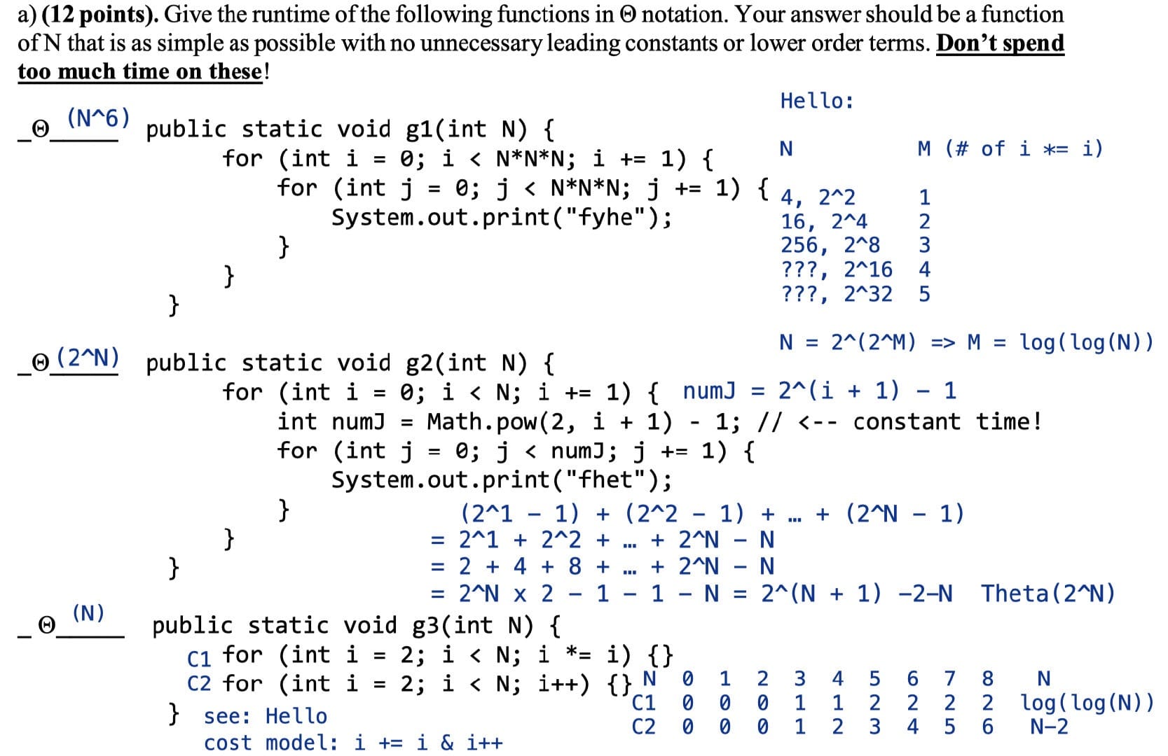
Note: i *= i => $\log{(\log{N})}$

Another way to think about the 3rd problem is that the first for-loop is less than $N$ and the second is approximately $N$, so it’s not necessary to compute C1.

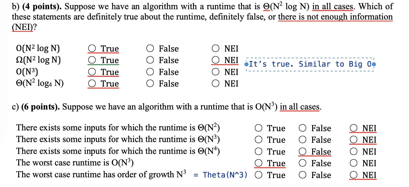
2. True or False:

3. Find the runtime of these two functions:

Assume $k(N)$ runs in constant time and returns a boolean.

public static void g4(int N) {
  if (N == 0) { return; }
  g4(N - 1);
  if (k(N)) { g4(N - 1); }
}

Worst case: $\Theta(2^N)$, when $k(N)$ always returns true.
Best case: $\Theta(N)$, when $k(N)$ always returns false.

public static void g5(int N) {
  if (N == 0) { return; }
  g5(N / 2);
  if (k(N)) { g5(N / 2); }
}

Worst case: $\Theta(N)$, when $k(N)$ always returns true.
Best case: $\Theta(\log{N})$, when $k(N)$ always returns false.

4. Find the runtime:

Assume HashSets use the idea of external chaining with resizing used in class, and that resize is linear.

public Set<Planet> uniques(ArrayList<Planet> x) {
  HashSet<Planet> items = new HashSet<>();
  for (int i = 0; i < x.size(); i += 1) { // N
    items.add(x.get(i)); // compute the hash code, best case: O(1)
  }
  return items;
}

Worst case: $\Theta(N^2)$, when elements are different and the array is always resizing.
Best case: $\Theta(N)$, when elements are all the same.

Marked: Worst case

Consider $x$ is a list of Strings. Suppose that the list contains $N$ strings, each of which is length $N$.

Worst case: $\Theta(N^3)$

String str = ...
// O(N^2) in worst case
for (String s : theChain) { // assume lengths are equal
  for (int i = 0; i < str.length; i += 1) {
    if (s.charAt(i) != str.charAt(i)) {
      break; // not equal
    }
  }
}

• All $N$ strings are different. In the function add(), it does comparison for [0, i) times. Since equality check for strings is linear time, so N-length strings need char-by-char equality check which takes $\Theta(N)$ time.

Best case: $\Theta(N)$

Ex 4 (Combo #3)

From: Spring 2017 Midterm #2

public static void f4(int N) {
  if (N == 0) { return; }
  f4(N / 2);
  f4(N / 2);
  f4(N / 2);
  f4(N / 2);
  g(N);         // runs in (N^2) time.
}

Note: f4() is constant time $\Theta(1)$. g() is quadratic $O(N^2)$.

// Recursion Tree
1.        N            4^0 x N^2
      / |   |  \
2.  N/2 N/2 N/2 N/2    4^1 x (N/2)^2 = 4^1 x N^2 / 4^1
   /||\ ...     /||\
3. N/4 ...             4^2 x (N/4)^2 = 4^2 x N^2 / 4^2
   ...
~N.                    4^lgN x (N/?)^2 = 4^lgN x N^2 x 4^lgN

Sum: $\Theta(N^2\log{N})$

Also, the recurrence is $T(N) = 4T(N/2) + N^2$.

According to the master theorem in case 2, the runtime is $T(N) = N^2 \log{N}$.

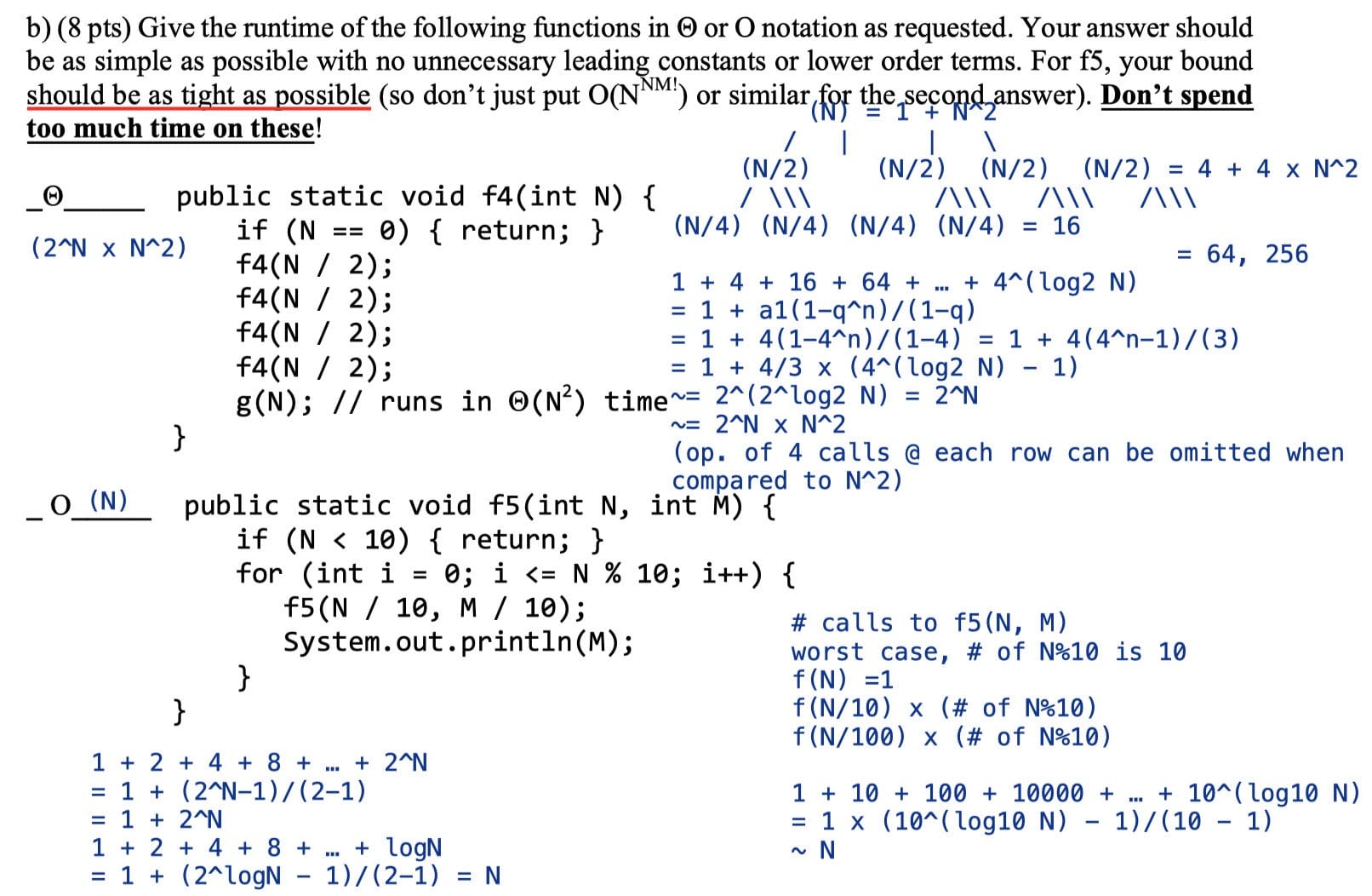
public static void f5(int N, int M) {
  if (N < 10) { return; }
  for (int i = 0; i < N % 10; i++) {
    f5(N / 10, M / 10);
    System.out.println(M);
  }
}

The recursion tree:

Cost model: println
// M does not affect the analysis, could be omitted
         f5(N, M)                  => N %10
         /  | ... \ x N %10
    f5(N/10)  ... f5(N/10)         => (N/10) %10
    /               x (N/10) %10
f5(N/10/10) ...                    => (N/10/10) %10
  /
...
/
f5(N/(10^lgN)) ...                 => (N/(10^lgN)) %10
Height: log10 (N)

Sum:

$$
\begin{aligned}
T(N) &= \Theta(\frac{N}{10^0} \mod 10 + \frac{N}{10^1} \mod 10 + \ldots + \frac{N}{10^{\log{N}}} \mod 10) \
&= \Theta(1\times N) = \Theta(N)
\end{aligned}
$$

Since each term is between $[0, 10)$, we can treat it as a constant.

Ex (Discussion 7, Spring 19)

Give the worst case and best case runtime in $\Theta(\cdot)$ notation.

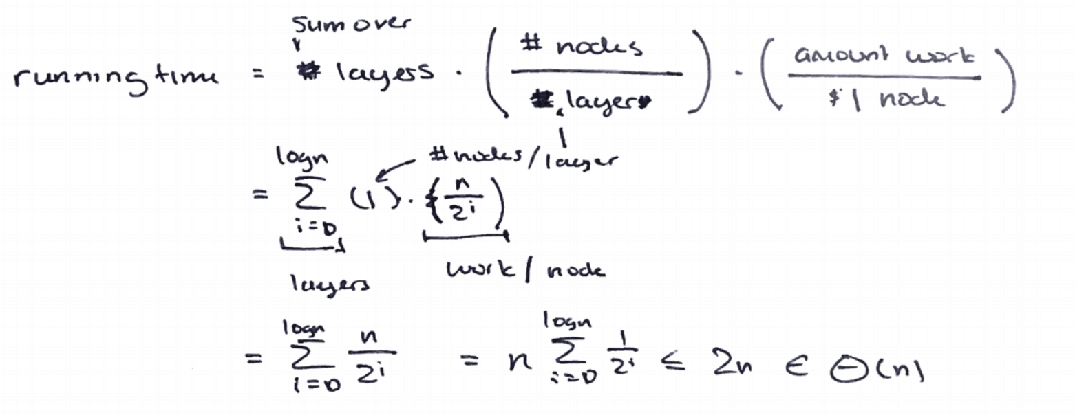
Ex 1 (andslam)

public void andslam(int N) {
  if (N > 0) {
    for (int i = 0; i < N; i += 1) {
      System.out.println("datboi.jpg");
    }
    andslam(N / 2);
  }
}

The recursion tree:

// cost model: println
          a(N)   => N   \
          /              \
      a(N/2)     => N/2   \
      /                    \ height = log N
  a(N/4)         => N/4    /
    /                     /
  ...                    /
  /                     /
a(1)             => 1  /

Sum: $\sim 2N - 1$

Worst case: $\Theta(N)$
Best case: $\Theta(N)$

In both cases the runtime is $\sum^{\log(N)}{i=0} \frac{N}{2^i} \leq N \sum^{\log(\infty)}{i=0} \frac{1}{2^i} = 2N$.

$$1 + \frac{1}{2} + \frac{1}{4} + \frac{1}{8} + \ldots + \frac{1}{N} \rightarrow 2$$

One potentially tricky portion is that $\sum^{\log(n)}_{i=0}\frac{1}{2^i}$ is at most $2$ because the geometric sum as it goes to infinity is bounded by $2$.

61B Style:

The TA demonstrates a general model to solve this kind of problems.

Steps:

• Height of Tree (layers)
  • $h = \log N$
• Branching Factor (#node = #subproblem)
  • Note each time andslam() is called, it makes 1 recursive call on n/2
  • #node per layer is 1
• Amount of Work each node / layer does ($f(N) = D(N) + C(N)$)
  • Sometimes it includes println, merging and combining time, etc.

Ex 2 (andwelcome)

public static void andwelcome(int low, int high) {
  System.out.print("[");
  for (int i = low; i < high; i += 1) {
    System.out.print("loyal "); // O(N)
  }
  System.out.println("]");
  if (high - low > 0) {
    double coin = Math.random(); /* 0 ~ 1 */
    if (coin > 0.5) {
      andwelcome(low, low + (high - low) / 2);  // f(N/2)
    } else { 
      andwelcome(low, low + (high - low) / 2);  // f(N/2)
      andwelcome(low + (high - low) / 2, high); // f(N/2)
    }
  }
}

Cost model: print("loyal ")

#layer: $\log N$
#node: $1$ or $2^i$
Amount of work: $N$ (all nodes)

Worst case: $\Theta(N \log N)$ , if there is no print: $\Theta(N)$
Best case: $\Theta(N)$, if there is no print: $\Theta(\log{N})$

Note: If amount of work equals $1$, the best-case running time will be $\Theta(\log N)$, just like the running time of binary search.

Ex 3 (spacejam)

public static void spacejam(int N) {
  if (N <= 1) {
    return;
  }
  for (int i = 0; i < N; i += 1) {
    spacejam(N - 1);
  }
}

Cost model: spacejam()

The recursion tree:

            s(N)               => N calls to s()
        /  |   ...   \
  s(N-1)  s(N-1)  ... s(N-1)   => N x (N-1) calls
    /   ...   |    ...
s(N-2) ...        ... s(N-2)   => N x (N-1) x (N-2) calls

............................   => ~N! calls
Height: N

#layer: $N$
#node: $\frac{N!}{(N - i)!}$
i = 1: N
i = 2: (N - 1) x N
i = 3: (N - 2) x (N - 1) x N
i = 4: (N - 3) x (N - 2) x (N - 1) x N
…
i = N: N!
Amount of work: $O(1)$

Worst case: $\sum^{N}_0 \frac{N!}{(N - i)!}\times 1 \sim N \times N! \in O(N \times N!)$
Best case: $O(N \times N!)$

Actually, calculating the sum of $\frac{N!}{(N-i)!}$ is a bit tricky because there is a pesky $(N-i)!$ term in the denominator. We can upper bound the sum by just removing the denominator, but in the strictest sense we would now have a $O$ bound instead of $\Theta$.

Ex (Examprep 7)

Ex 1 (p/r/s)

What is the worst-case runtime for $p(N)$? Assume $h$ is a boolean function requiring constant time.

int p(int M) {
  return r(0, M);
}

int r(int i, int M) {     // O(M - i) in worst case. Since i = 0, O(M)
  if (i >= M) return 0;   // assume false
  if (s(i) > 0) return i; // assume false, s(i) takes O(i)
  return r(i + 1, M);     // go deep
}

int s(int k) {            // O(k) in worst case
  if (k <= 0) return 0;
  if (h(k)) return k;     // assume h(k) => false
  return s(k - 1);        // go deep
}

The recursion tree:

p(M):
           r(0, M)    => s(0) => O(0)    \
             /                            \
         r(1, M)      => s(1) => O(1)      \
           /                                \
       r(2, M)        => s(2) => O(2)        \ height = M = N
        /                                    /
      ...                                   /
      /                                    /
r(M-1, M)             => s(M-1) => O(M-1) /

Worst case: $\Theta(N^2)$

Ex 2 (M/L/U)

What is the worst-case runtime of $p(N)$? Assume that calls to $h$ require constant time.

void p(int M) {
  int L, U;
  for (L = U = 0; U < M; L += 1, U += 2) { // U < M, U += 2 => M / 2 ~ M
    for (int i = L; i < U; i += 1) {
      h(i);
    }
  }
}

Cost model: h()

L	0	1	2	3	4	5	6	7	8	9
U	0	2	4	6	8	10	12	14	16	18
U-L	0	1	2	3	4	5	6	7	8	9

Worst-case: $\Theta(N^2)$

Disjoint Sets

Two sets are named disjoint sets if they have no elements in common. A Disjoint Set (or Union-Find) data structure keeps track of a fixed number of elements partitioned into a number of disjoint sets.

1. connect(x, y): connect $x$ and $y$. Also known as union
2. isConnected(x, y): returns true if $x$ and $y$ are connected (i.e. part of the same set).

Goal: Design an efficient disjoint set implementation.

• Number of elements $N$ can be huge.
• Number of method calls $M$ can be huge.
• Calls to methods may be interspersed (invoking order).

The Naive Approach:

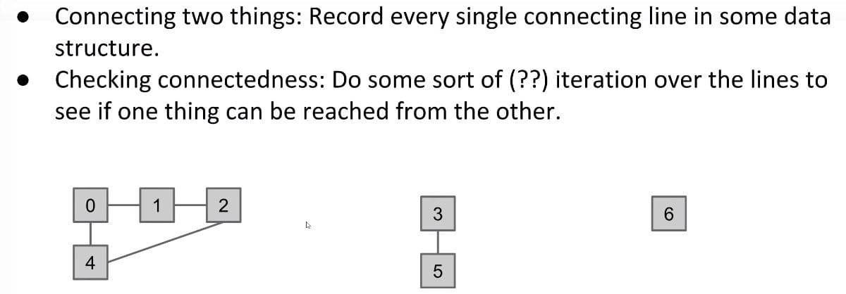
The Better Approach:

Connected Components. Rather than manually writing out every single connecting line, only record the sets that each item belongs to. In other words, we only need to keep track of which connected component each item belongs to.

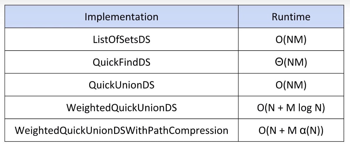
This chapter will be a chance to see how an implementation of a data structure evolves. We will discuss four iterations of a Disjoint Set design before being satisfied:

• ListOfSets
• Quick Find
• Quick Union
• Weighted Quick Union (WQU)
• Weighted Quick Union with Path Compression (WQU-PC)

We will see how design decisions greatly affect asymptotic runtime and code complexity.

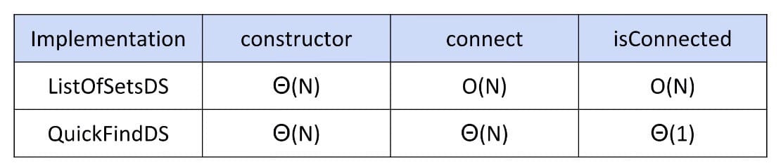
ListOfSets

Intuitively, we might first consider representing a disjoint set as a list of sets, e.g, List<Set<Integer>>.

For instance, if we have $6$ elements and nothing has been connected yet, our list of sets looks like: [{0}, {1}, {2}, {3}, {4}, {5}, {6}]. Looks good. However, consider how to complete an operation like connect(5, 6). We’d have to iterate through up to $N$ sets to find $5$ and $N$ sets to find $6$. Our runtime becomes O(N).

The lesson to take away is that initial design decisions determine our code complexity.

Quick Find

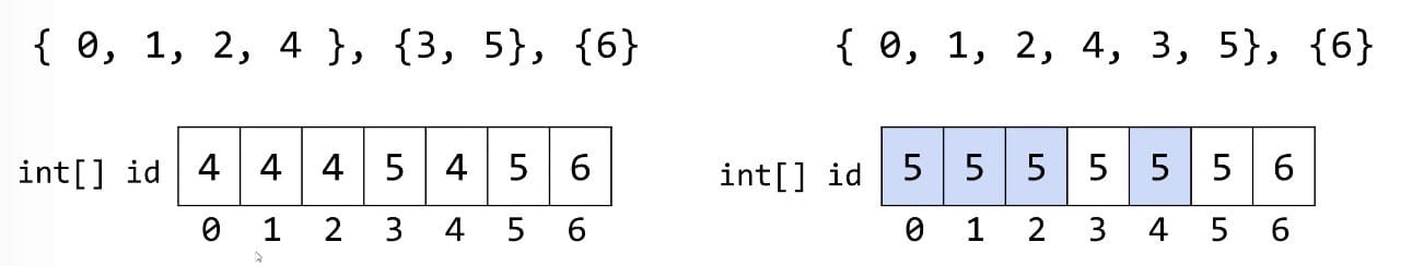
public class QuickFindDS implements DisjointSets {
  private int[] id;

  // O(1)
  public boolean isConnected(int p, int q) {
    return id[p] == id[q];
  }

  // Need to iterate through the array => O(N)
  public void connect(int p, int q) {
    int pid = id[p];
    int qid = id[q];
    for (int i = 0; i < id.length; i++) {
      if (id[i] == pid) {
        id[i] = qid;
      }
    }
  }
}

Having to create $N$ distinct sets initially is $\Theta(N)$.

Quick Union

Quick Find’s bad feature: Connecting two sets is slow (need much checking and updating)!

We’ve changed so many values in Quick Find.

Hard question: How could we change our set representation so that combining two sets into their union requires changing one value?

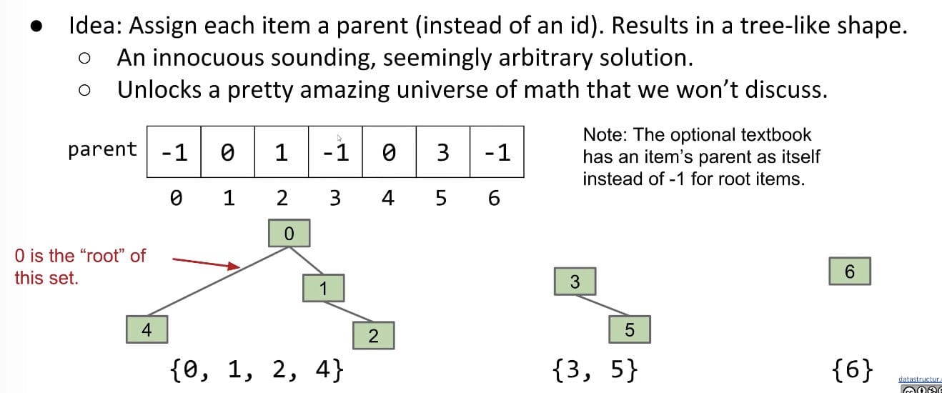
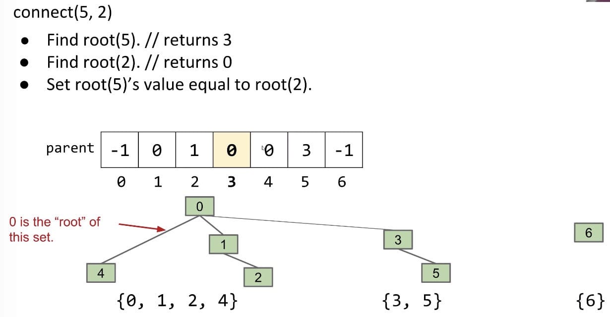
public class QuickUnionDS implements DisjointSets {
  private int[] parent;

  public QuickUnionDS(int N) {
    parent = new int[N];
    for (int i = 0; i < N; i += 1) {
      parent[i] = -1;
    }
  }

  private int find(int p) { /* root() */
    int r = p;
    while (parent[r] >= 0) {
      r = parent[r];
    }
    return r;
  }

  @Override
  public boolean isConnected(int p, int q) {
    return find(p) == find(q);
  }

  @Override
  public void connect(int p, int q) {
    int i = find(p);
    int j = find(q);
    parent[i] = j;
  }
}

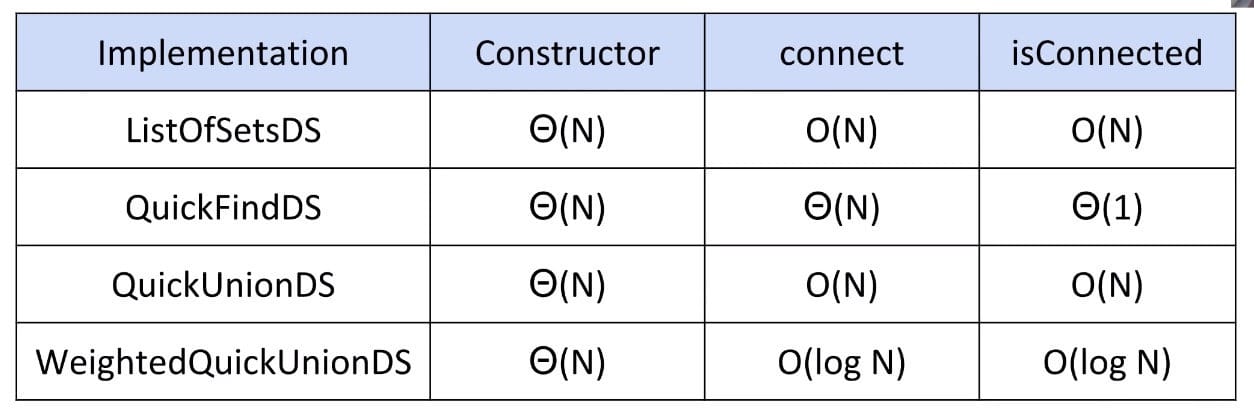
Runtime Table:

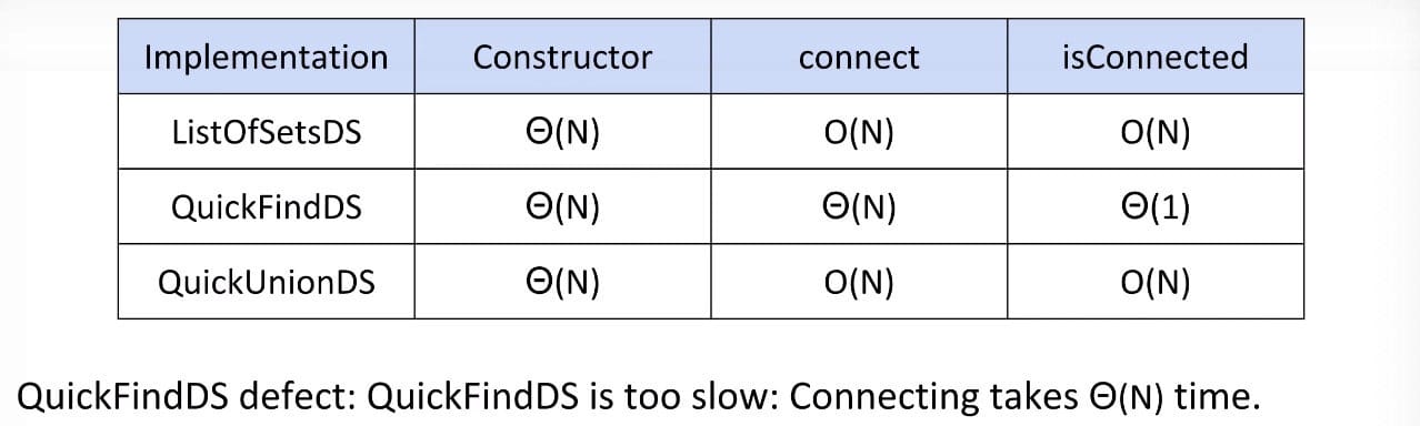
Defect: Trees can get tall. Results in potentially even worse performance than QuickFind if tree is imbalanced since isConnected does not take constant time.

Things would be fine if we just kept our tree balanced.

Weighted Quick Union

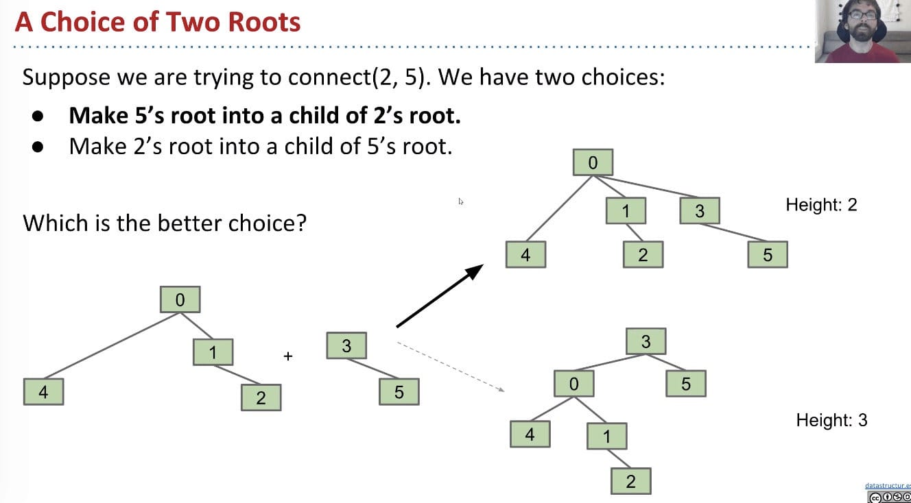
Modify quick-union to avoid tall trees.

• Track tree size (number of elements)
• New Rule: Always link root of a smaller tree to a larger tree (weight, not height).

connect(int p, int q) needs to somehow keep track of sizes. Two common approaches:

1. Use values other than -1 in parent array for root nodes to track size
2. Create a separate size array. (algs4)

Note: If every time it just connects one item, it would be great (the height keeps small).

private int find(int p) { /* root() */
  int r = p;
  while (parent[r] >= 0) {
    r = parent[r]; // O(log N)
  }
  return r;
}

@Override
public boolean isConnected(int p, int q) {
  return find(p) == find(q); // O(log N)
}

@Override
public void connect(int p, int q) {
  int i = find(p); // O(log N)
  int j = find(q); // O(log N)
  parent[i] = j;   // O(1)
}

Path Compression

Another clever idea when doing find:

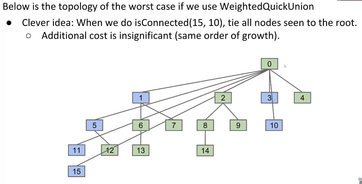
/* Set to next.next */
private int find_better_1(int p) { /* root() */
  int r = p;
  while (parent[r] >= 0) {
    int temp = r;
    r = parent[r];
    if (parent[r] >= 0) { /* == temp.next.next */
      parent[temp] = r; /* In case we set it to -1. It already points to root */
    }
  }
  return r;
}

/* Point to root (The lecture uses this method) */
private int find_better_2(int p) {
  int r = p;
  while (parent[r] >= 0) {
    r = parent[r];
  }
  /* Set related parents to root  - Same order of growth */
  int root = r;
  r = p; /* reset */
  while (parent[r] >= 0) {
    int temp = r;
    r = parent[r]; /* next */
    parent[temp] = root;
  }
  return r;
} /* O(log N) x 2 */

Recall that both connect(x, y) and isConnected(x, y) always call find(x) and find(y). Thus, after calling connect or isConnected enough, essentially all elements will point directly to their root.

By extension, the average runtime of connect and isConnected becomes almost constant in the long term! This is called the amortized runtime.

Technically, the order of growth of this data structure becomes $O(N + M lg* N)$.

lg* N, aka. the iterated logarithm, is less than 5 for any realistic input.

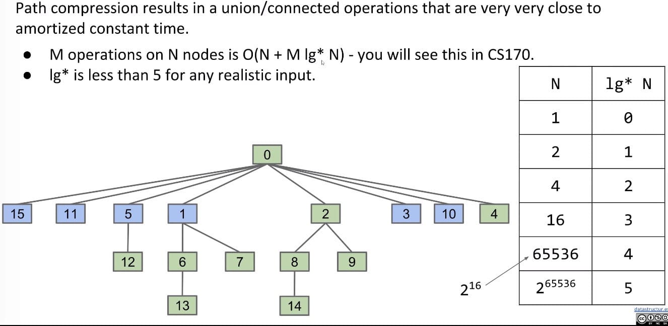
Actually, there is a tighter bound: $O(N + M\alpha(N))$, where $\alpha$ is the inverse Ackermann function which is less than 5 for all practical inputs!

Done

The end result of our iterative design process is the standard way disjoint sets are implemented today - quick union and path compression (once you have path compression, you don’t need weighted quick union).

Implementation

• Lab 6 - UnionFind.java (with PC)
• Princeton - WeightedQuickUnionUF.java

HW 2: Percolation

HW 2: Percolation

My Implementation

Idea:

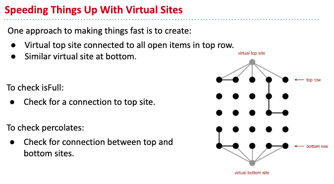
Backwash Problem (isFull(row, col)):

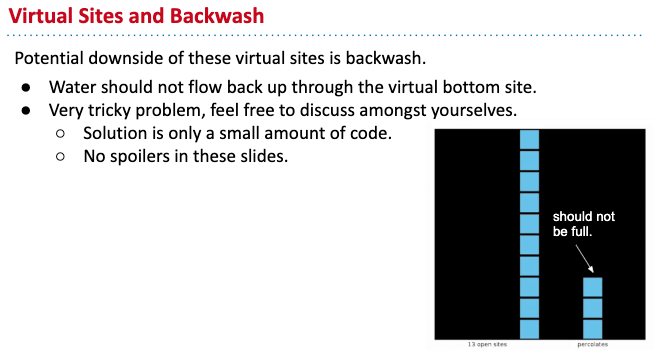
Solution: Use two WeightedQuickUnionUFs (one with only top entry, the other one with both top and bottom entries)

Possible Solution (Online): One additional N by N grid to store states