CS 61B | Part 13 | Bubble & Quick Sort, Stability, Bounds, Radix Sort, Comparisons

Bubble Sort

Idea

Reference: wiki

Bubble sort (or sinking sort) is a simple sorting algorithm that repeatedly steps through the list, compares adjacent pairs and swaps them if they are in the wrong order. The pass through the list is repeated until the list is sorted.

Although the algorithm is simple, it is too slow and impractical for most problems even when compared to insertion sort.

Bubble sort can be practical if the input is in mostly sorted order with some out-of-order elements nearly in position.

Code

/* Bubble Sort */
                      N-1
Pivot:     <-----------i
Index:  0 [1] 2  3  4 [5]
Data:   3  9  5  2  1  8
        j----------->
        j>

public static void bubbleSort(int[] a) {
  int N = a.length;
  for (int i = N - 1; i > 0; --i) { // i >= 0 --> OK
    for (int j = 0; j < i; ++j) {
      if (a[j] > a[j + 1]) {
        swap(a, j, j + 1);
      }
    }
  }
}

Quick Sort

Backstory

Invented by Sir Tony Hoare in 1960, at the time a novice programmer.

Quicksort was the name chosen by Tony Hoare for Partition Sort. For most common situations, it is empirically the fastest sort. He was lucky that the name was correct.

Problem:

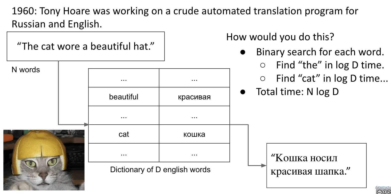
Limitation at the time:

• Dictionary stored on long piece of tapes, sentence is an array in RAM.
  • Binary search of tapes is not log time (requires physical movement).
• Better Approach: Sort the sentence and scan dictionary tape once. Takes $N\log{N} + D$ time.
  • Bubble Sort
  • Quick Sort

Partitioning

Interview Question:

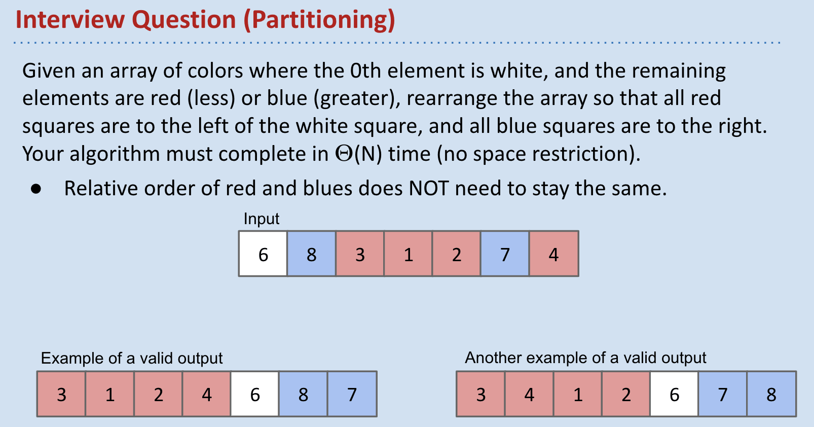
Approach 1: Scan from the right edge of the list.

• If anything is smaller, stick it in the leftmost.
• If anything is larger, skip it.
• Very natural use for a double ended queue.

Approach 2: Insert $6$ into a BST, then 8, 3, …, 4.

• All the smaller items are on the left.
• All the larger items are on the right.

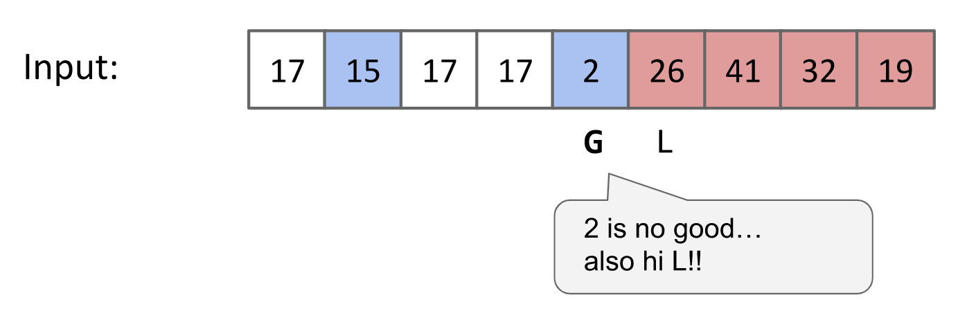
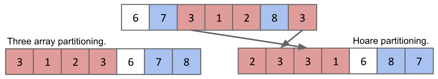
Approach 3: Create another array. Scan the original array 3 times.

• 1st Scan: Copy all red items to the first $R$ spaces.
• 2nd Scan: Copy the white item.
• 3rd Scan: Copy all blue items to the last $B$ spaces.

Idea

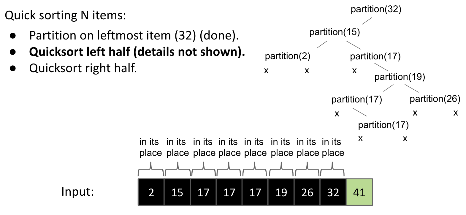
Quicksorting $N$ items:

• Partition on leftmost item. (one of many versions)
• Quicksort left half.
• Quicksort right half.

Demo: link

Runtime

Fastest Sort

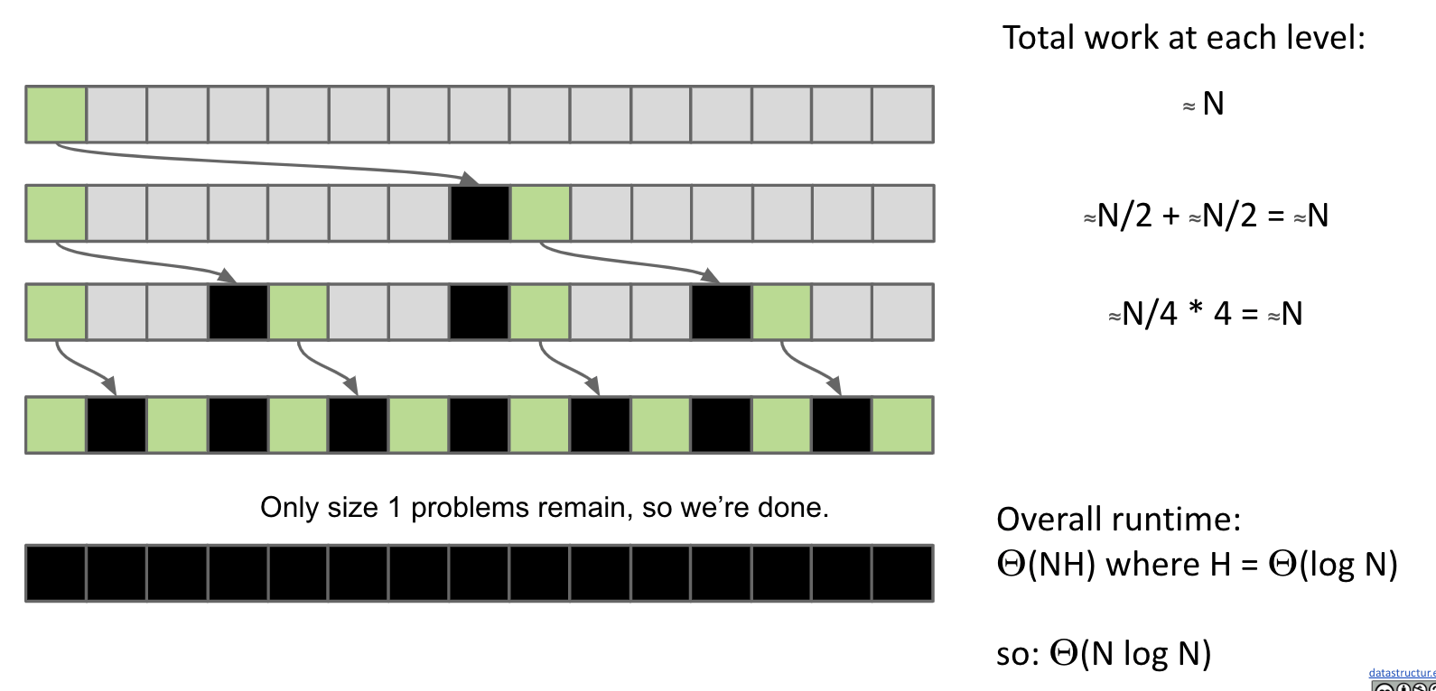
Partitioning takes $\Theta(K)$ time, where $K$ is the number of elements being partitioned.

Interesting Twist: Overall runtime will depend crucially on where pivot ends up.

Best Case: Pivot Always Lands in the Middle. ==> $\Theta(N\log{N})$

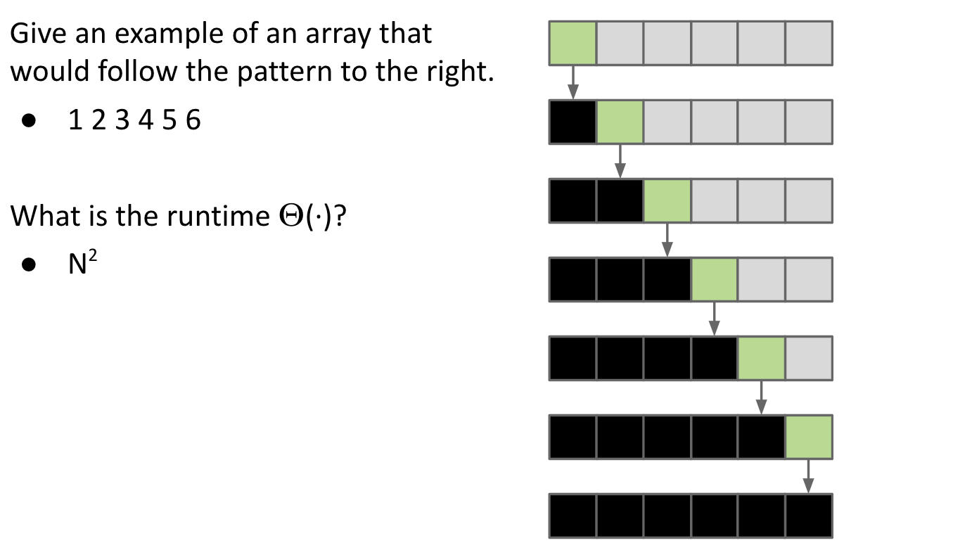
Worst Case: Pivot Always Lands at the Beginning. ==> $\Theta(N^2)$

In summary:

• Best Case: $\Theta(N\log{N})$
• Worst Case: $\Theta(N^2)$
  • For our pivot strategy: Sorted or almost sorted.
    • It can be improved by randomly pick the pivot.
• Randomly chosen array case: $\Theta(N\log{N})$
  • With extremely high probability!

Compare this to Mergesort:

• Best Case: $\Theta(N\log{N})$
• Worst Case: $\Theta(N\log{N})$

Recall that linearithmic vs. quadratic is a really big deal. So how can Quicksort be the fastest sort empirically?

The answer: It takes $\Theta(N\log{N})$ on average.

Note: Rigorous proof requires probability theory + calculus, but intuition + empirical analysis will be convincible.

Argument

Argument 1: 10% Case

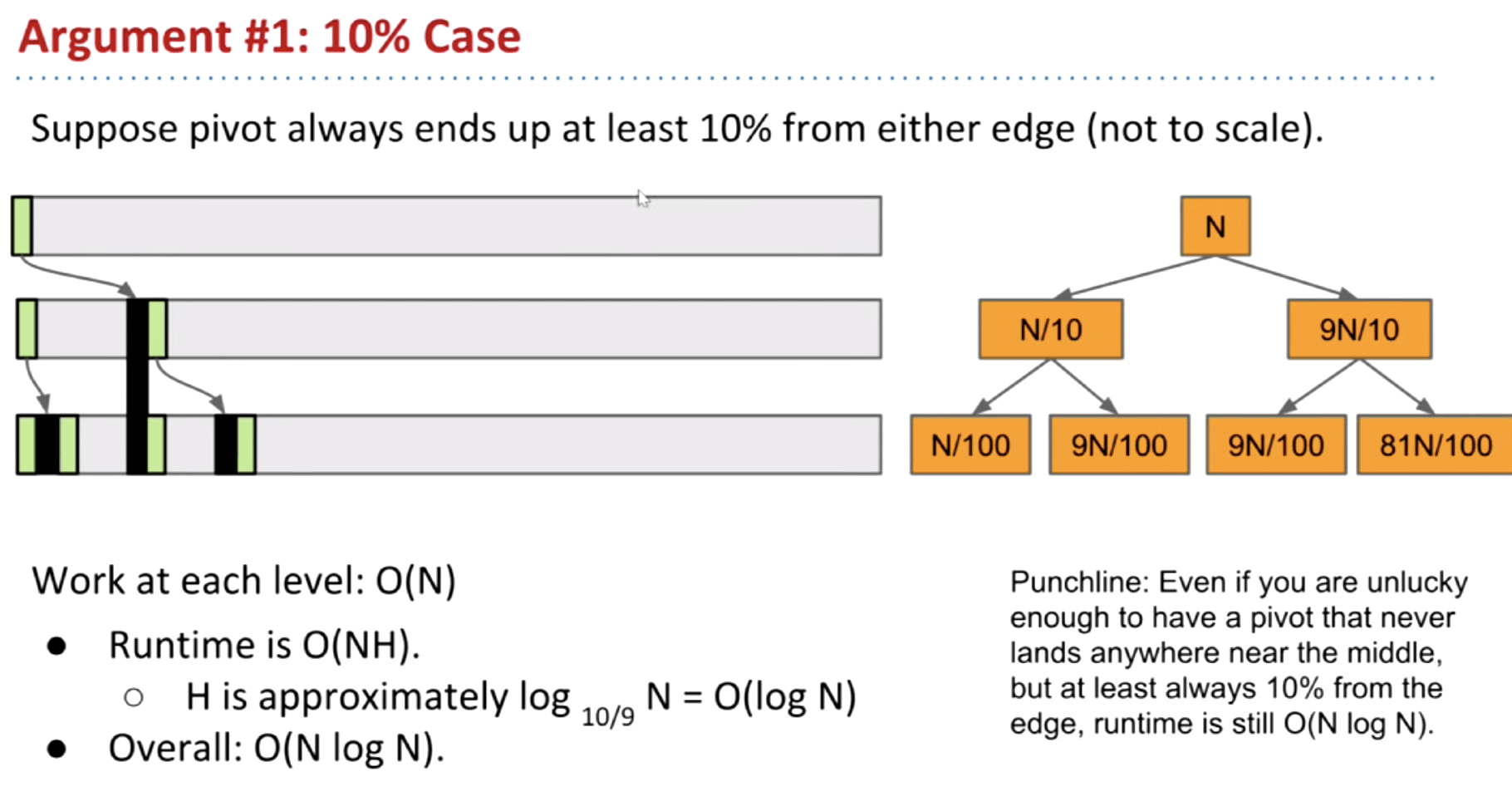
Punchline: Even if you are unlucky enough to have a pivot that never lands anywhere near the middle, but at least always 10% from the edge, runtime is still $O(N\log{N})$.

Argument 2: Quicksort is BST sort (Gez!)

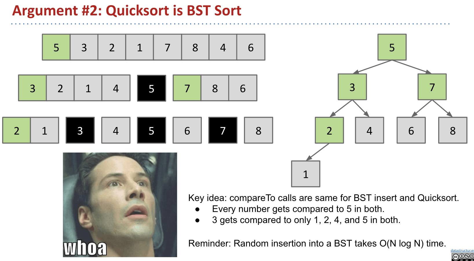
Note: Whenever comparison happens in your partition, think of the comparison and insertion processes in BST. Also, notice that the worst case in BST insertion is $\Theta(N)$.

Argument 3: Empirical Quicksort Runtimes

For $N$ items:

• Average number of compares to complete Quicksort: $\sim 2N \ln{N}$
• Standard deviation: $\sqrt{(21-2\pi^2)/3}N \approx 0.6482776N$

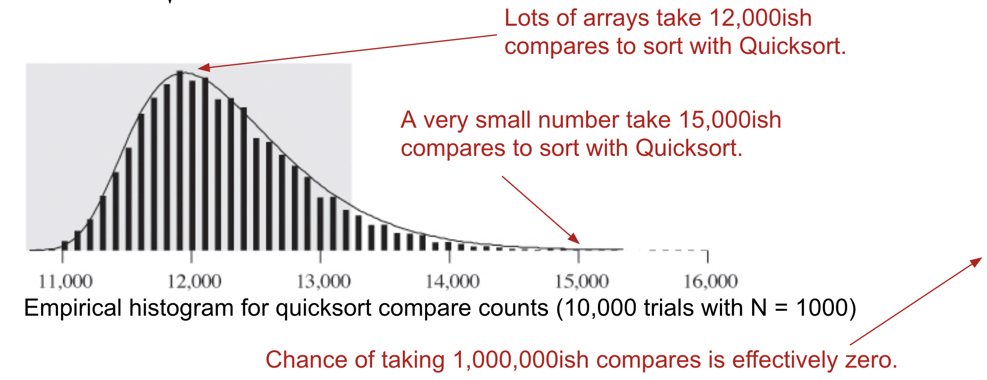
Note: It means the probability of worst case is quite low.

Avoid Worst Case

If pivot always lands somewhere “good”, Quicksort is $\Theta(N\log{N})$. However, the very rare $\Theta(N^2)$ cases do happen in practice.

• Bad Ordering: Array already in sorted order (or almost sorted order).
• Bad Elements: Array with all duplicates.

Based on our version of Quicksort, we have the two properties:

• Leftmost item is always chosen as the pivot.
• Our partitioning algorithm preserves the relative order of $\leq$ and $\geq$ items.

Actually, we can embrace these four philosophies:

1. Randomness: Pick a random pivot or shuffle before sorting (good!).
2. Smarter pivot selection: Calculate or approximate the median.
3. Introspection: Switch to a safer sort if recursion goes to deep.
4. Preprocess the array: Could analyze array to see if Quicksort will be slow, but no obvious way to do this.

1. Randomness

Dealing with bad ordering:

• Strategy #1: Pick pivots randomly.
• Strategy #2: Shuffle before you sort.
  • The 2nd strategy requires care in partitioning code to avoid $\Theta(N^2)$ behavior on arrays of duplicates.
  • Common bug in textbooks! See A level problems.

2. Smarter Pivot Selection

Constant time pivot pick:

What about:

• Picking the 8th pivot?
• Picking the first, last, and the middle pivots, and compute the median?

Sounds good. However, for any pivot selection procedure that is:

• Deterministic
• Constant time

There exists an input that will cause that Quicksort to take $\Theta(N^2)$.

Note: In fact, Java Quicksort is non-random. You can give an array of integers and cause it to crash because the recursion depth goes too deep.

But it happens rarely and getting random numbers can be expensive.

Linear time pivot pick:

We could calculate the actual median in $\Theta(N)$.

It turns out the worst case is $\Theta(N\log{N})$, but it is slower than Mergesort, according to computational experiments.

3. Introspection

We can also simply watch the recursion depth. If it exceeds some critical value (say $10\ln{N}$), switch to Mergesort or Selection Sort.

Perfectly reasonable approach, though not super common in practice.

4. Preprocess the Array

There may be no obvious way to do this.

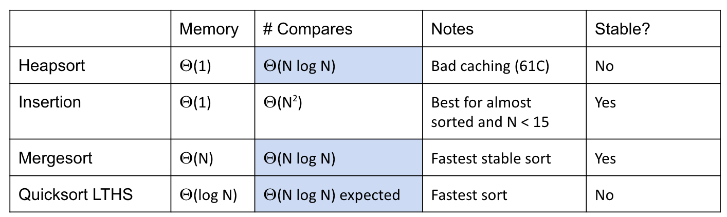
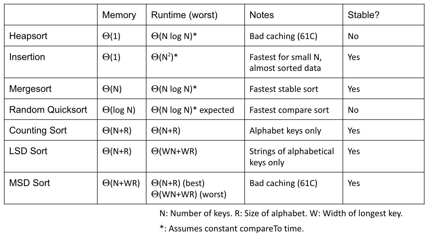
Sorting Summary (So far):

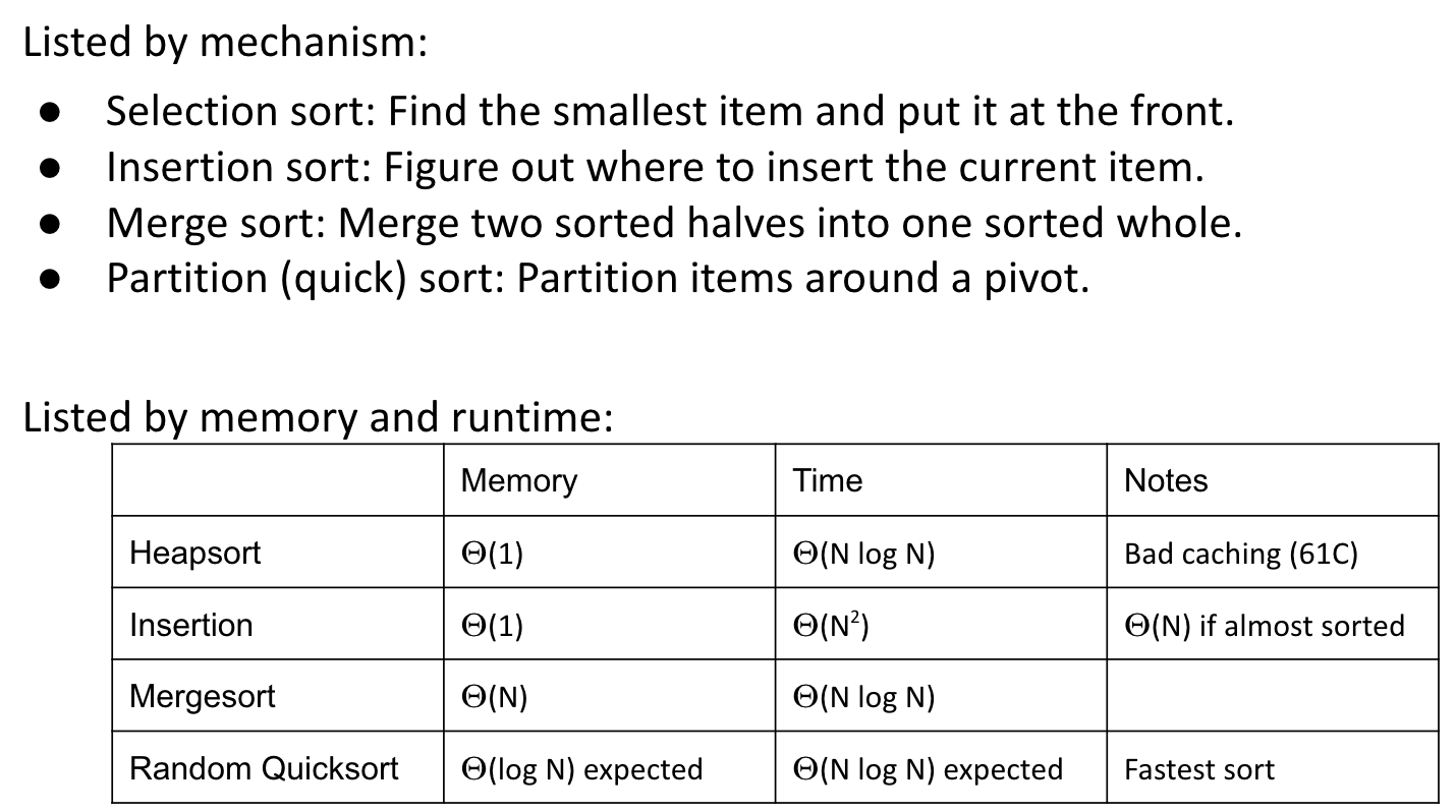
Note: Heapsort has bad caching performance, basically because it’s jumping all over the place (sinking) to find children or parents.

In-place Partition

Better Scheme: Tony originally proposed a scheme called Hoare's Partitioning where two pointers walk towards each other.

Hoare’s Partitioning:

Two Pointers: Left and right pointers work for the pivot.

• Left pointer i loves small items, and hates large or equal items.
• Right pointer j loves large items, hates small or equal items.
• Stop at a hated item.

Walk towards each other, swapping anything they hate.

• When both pointers have stopped, swap and move pointers by one.
• When pointers cross, it’s done.
• Swap pivot with the right pointer j.

Note:

• Hating equal items is necessary when we have an array of many duplicate items.

  piv                  j<-j
  6  6  6  6  6  6  6  6  6
     i------------------->i
  ^                    ^
  ---------------------- Swap  

• The partition scheme is independent of the choice of the pivot. If we pick a pivot in the middle, we can just swap it with the leftmost item at the beginning.

If you find yourself in a funny case, get yourself into a case you understand and then it’ll be okay.

Demo: link

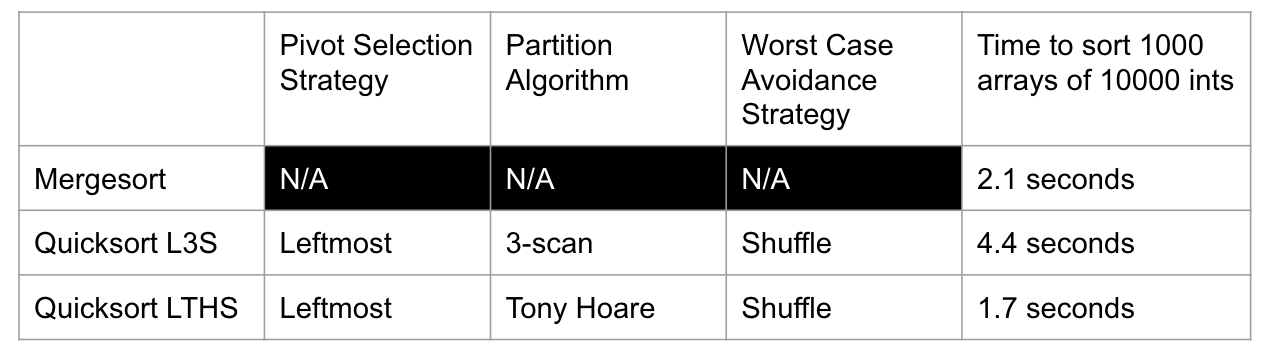
Compare to Mergesort:

Using Tony Hoare’s two pointer scheme, Quicksort is better than Mergesort!

Code

Okay Version

Caveat:

         i/j
data: 2  5 
         j  i    // i moves first
data: 2  5

Note: It’s not good. Bad Case: Duplicate items => O(N^2)

public static void quicksort(int[] a) {
  if (a == null || a.length == 0) return;
  // StdRandom.shuffle(a);
  quicksort(a, 0, a.length - 1);
}
//  0  1  2  3  4        0  1  2  3  4        0  1  2  3  4
//  1  9  3  4  6   =>   1  9  3  4  6   =>   1  6  3  4  9
//  p  i        j           p  i     j           p  i  j
//  j<-----------              -------->i           ----->i
private static void quicksort(int[] a, int lo, int hi) {
  if (lo >= hi) return;  // size == 1

  int p = lo;  // pivot
  int i = lo + 1, j = hi;
  while (true) {
    while (i <= j && a[i] <= a[p]) ++i;  // i moves
    while (i <= j && a[j] >= a[p]) --j;  // j moves
    if(i > j) break;
    swap(a, i, j);             // swap i, j
  }

  swap(a, p, j);  // swap pivot, j
  quicksort(a, lo, j - 1);
  quicksort(a, j + 1, hi);
}

Algs4 Version

Caveat:

Some of them are from algs4.

• Two pointers should move first and then compare. For example, if we’ve exchanged i and j, we want to move on to new values in the next round.
• Staying in bounds. If the smallest item or the largest item in the array is the partitioning item, we have to take care that the pointers do not run off the left or right ends of the array, respectively.
  • Our partition() implementation has explicit tests to guard against this circumstance. The test (j == lo) is redundant, since the partitioning item is at a[lo] and not less than itself.
• Duplicate Keys: Handling items with keys equal to the partitioning item’s key. It is best to stop the left scan for items with keys greater than or equal to the partitioning item’s key and the right scan for items with key less than or equal to the partitioning item’s key. Even though this policy might seem to create unnecessary exchanges involving items with keys equal to the partitioning item’s key, it is crucial to avoiding quadratic running time in certain typical applications.

public static void qsort(int[] a) {
  qsort(a, 0, a.length - 1);
}

private static void qsort(int[] a, int lo, int hi) {
  if (lo >= hi) return;
  int j = partition(a, lo, hi);
  qsort(a, lo, j - 1);
  qsort(a, j + 1, hi);
}

private static int partition(int[] a, int lo, int hi) {
  int p = a[lo];
  int i = lo; int j = hi + 1;
  while (true) {
    while (a[++i] < p) {  // move i
      if (i == hi) break;
    }
    
    while (a[--j] > p) {  // move j
      if (j == lo) break; 
      // redundant since a[lo] acts as sentinel
    }

    if (i >= j) break; // check if pointers cross
    swap(a, i, j);
  }

  swap(a, left, j);
  return j;
}

Pivot Scheme (Median)

More recent pivot / partitioning schemes do somewhat better. Best known Quicksort uses a two-pivot scheme. This version was introduced to the world by a previously unknown guy, in a Java developers forum (link).

More Improvement: A much better approach could be to use the median as our pivot.

• Approach 1: Create a min heap and a max heap, and insert some yadda yadda.
• Approach 2: Build a balanced BST, and take the root, but it only works if the tree is perfectly balanced.
• Approach 3: Sort and take the middle. (X)

PICK

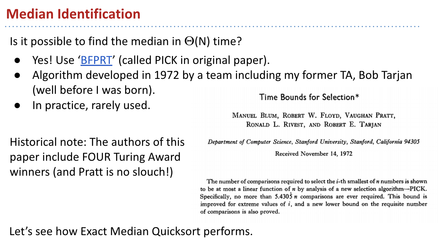
What happens if we use this algorithm in Quicksort?

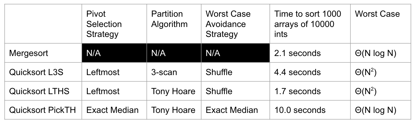
Cost to compute medians is too high. So, we have to live with worst case $\Theta(N^2)$ if we want good practical performance.

Quick Select

It turns out that partitioning can be used to find the exact median. The resulting algorithm is the best known median identification algorithm.

Demo:

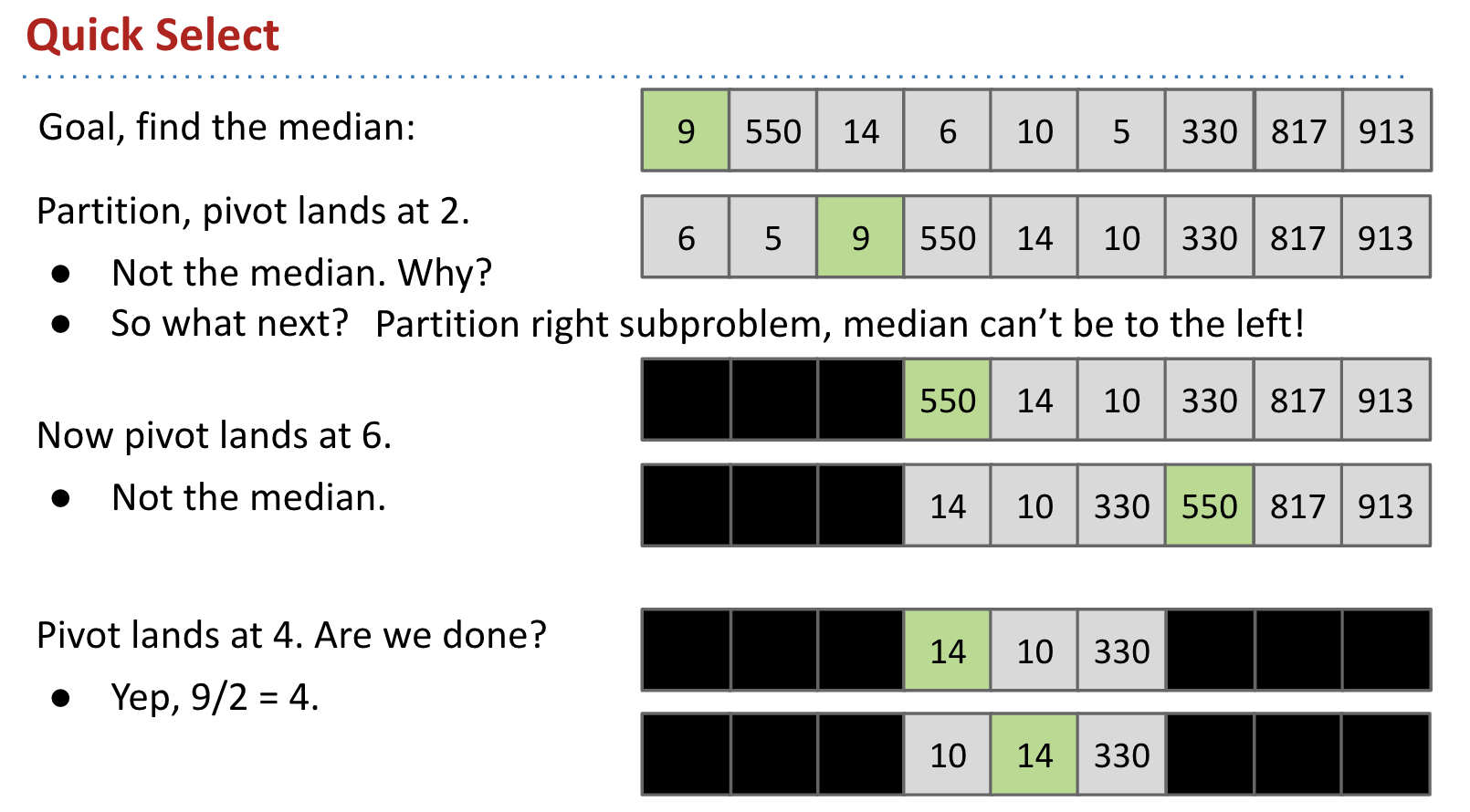
Runtime:

Worst case: $\Theta(N^2)$ occurs if array is in sorted order.

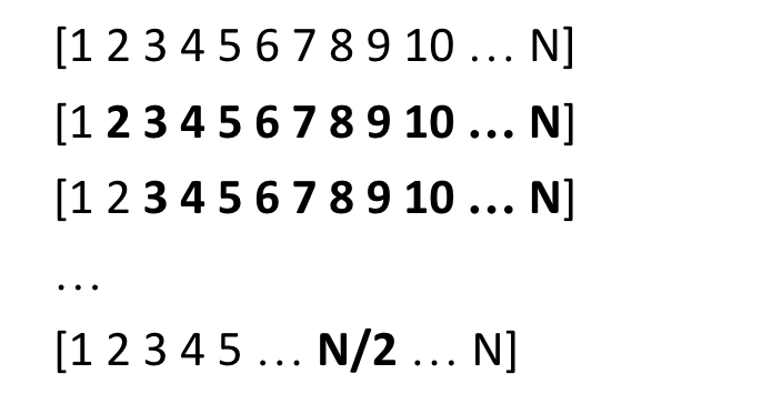
On average, Quick Select will take $\Theta(N)$ time.

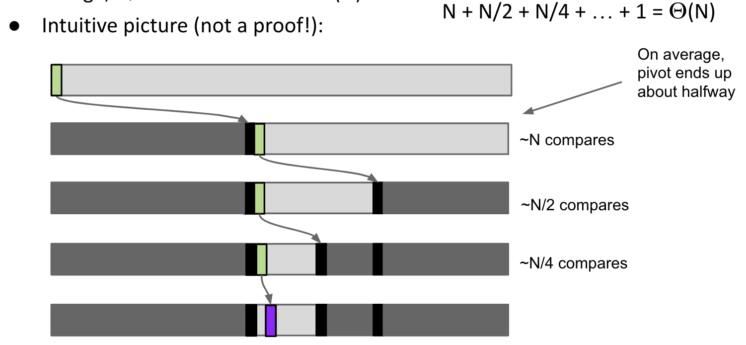
Although it is bound by $\Theta(N^2)$, it is better than PICK on average (just like Mergesort vs. Quicksort).

However, if we apply Quick Select to Quicksort, resulting algorithm is still quite slow. It is strange to do a bunch of partitions to identify the optimal item to partition around.

Property: Stability

Stable: Order of equivalent items is preserved.

Stable Example:

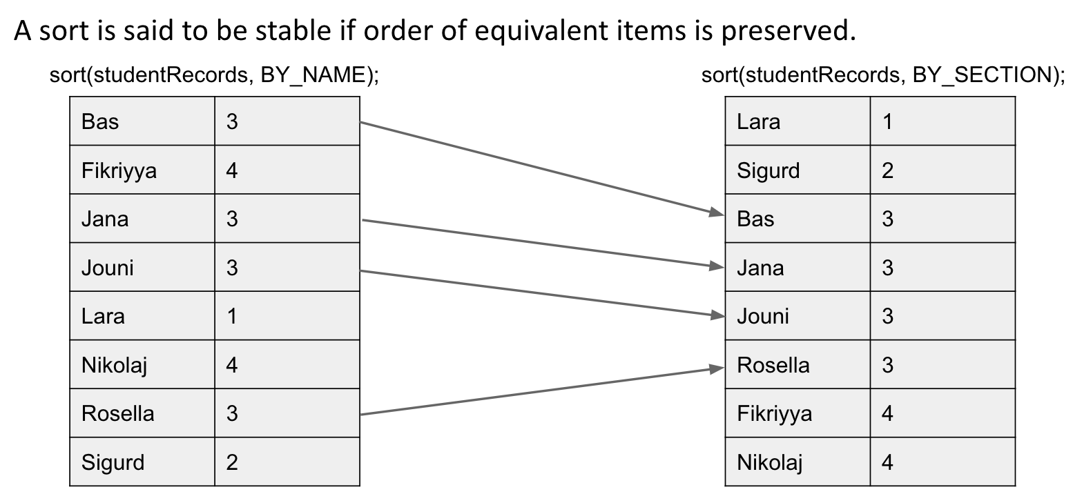
Note: Equivalent items don’t cross over when being stably sorted.

Unstable Example:

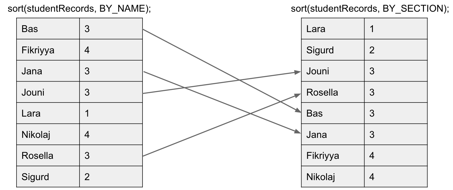
Sorting instability can be really annoying.

• Is insertion sort stable?

  Yes. Equivalent items never move past their equivalent brethren (= brothers).

• Is Quicksort stable?

  Depends on your partitioning strategy. Quicksort LTHS is not stable.

  

Besides, Heapsort is not stable. Mergesort is stable.

Java’s Example:

In Java, Arrays.sort() uses:

• Mergesort (specifically the TimSort variant) if someArray consists of Objects.
• Quicksort if someArray consists of primitives.

Why?

• When you are using a primitive value, they are the same. A 4 is a 4. Unstable sort has no observable effect.
• By contrast, objects can have many properties, e.g. section and name, so equivalent items can be differentiated.

Optimizing Sort Tricks

There are some additional tricks we can play:

• Switch to Insertion Sort:
  • When a subproblem reaches size 15 or lower, use insertion sort.
• Mark sort adaptive: Exploit existing order in array (Insertion Sort, Smoothsort, Timsort)
  • Timsort is a hybrid stable sorting algorithm derived from Mergesort and Insertion Sort. It is used in Python and Java.
• Exploit restrictions on set of keys. If number of keys is some constant, e.g. [3, 4, 1, 2, 4, 3, …, 2, 2, 2, 1, 4, 3, 2, 3], we can sort faster using 3-way quicksort.
  • Idea: Process all occurrences of pivot based on Duntch national flag (DNF) problem.

By the way:

Sorting is a fundamental problem on which many other problems rely.

• Sorting improves duplicate finding from a naive $N^2$ to $N\log{N}$.
• Sorting improves 3SUM from a naive $N^3$ to $N^2$.

Factorial & Linearithmic

Consider the functions $N!$ and $(N/2)^{N/2}$:

Is $N! \in \Omega((N/2)^{N/2})$?

Note:

• $\in \Omega$ can be informally interpreted as $\geq$.
• Or it means: Does factorial grow at least as quickly as $(N/2)^{N/2}$?

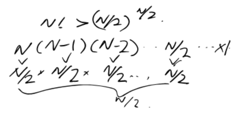
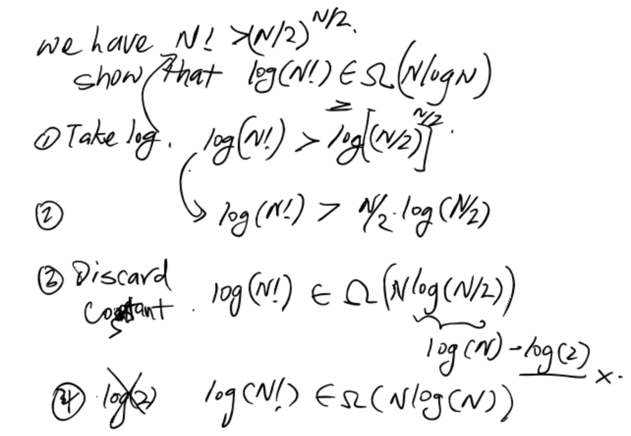
Given $N! > (N/2)^{N/2}$, show that $\log{(N!)} \in \Omega(N\log{N})$.

Now, show that $N\log{N} \in \Omega(\log{(N!)})$.

• $\log{(N!)} = \log{(N)} + \log{(N - 1)} + \log{(N-2)} + \ldots + \log{(1)}$
• $N\log{N} = \log{(N)} + \log{(N)} + \log{(N)} + \ldots + \log{(N)}$
• Therefore, $N\log{N} \in \Omega(\log{(N!)})$

Finally, we can say:

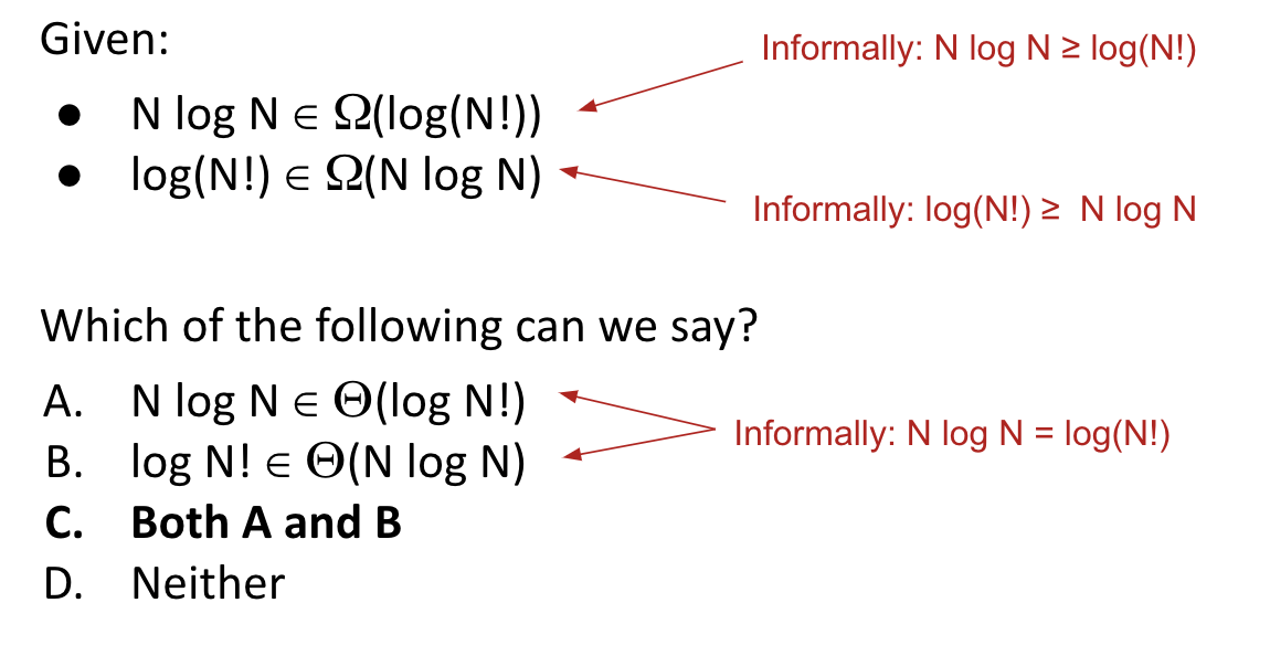
So, these two functions grow at the same rate asymptotically.

Algorithmic Bounds

Bound Definition

We have shown several sorts to require $\Theta(N\log{N})$ worst case time. Can we build a better sorting algorithm?

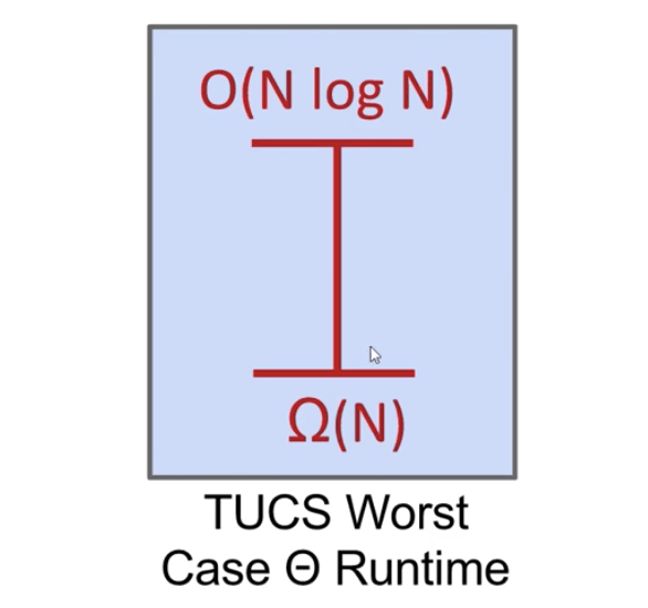
Let the ultimate comparison sort (TUCS) be the asymptotically fastest possible comparison sorting algorithm, possibly yet to be discovered.

Let $R(N)$ be its worst case runtime in $\Theta$ notation.

• Worst case runtime of TUCS, $R(N)$ is $O(N\log{N})$. Why? Because we have Mergesort.

We can also say:

• Worst case runtime of TUCS, $R(N)$ is $\Omega(1)$.

The problem doesn’t get easier with $N$. Can we make a stronger statement than $\Omega(1)$?

• Worst case runtime of TUCS, $R(N)$ is also $\Theta(N)$.

TUCS has to at least look at every item.

Can we make an even stronger statement on the lower bound of the worst case performance of TUCS?

With a clever statement, yes. It is $\Omega(N\log{N})$.

This lower bound means that across the infinite space of all possible ideas that any human might ever have for sorting using sequential comparison, none has a worst case runtime that is better than $N\log{N}$.

The intuitive explanation is as followed.

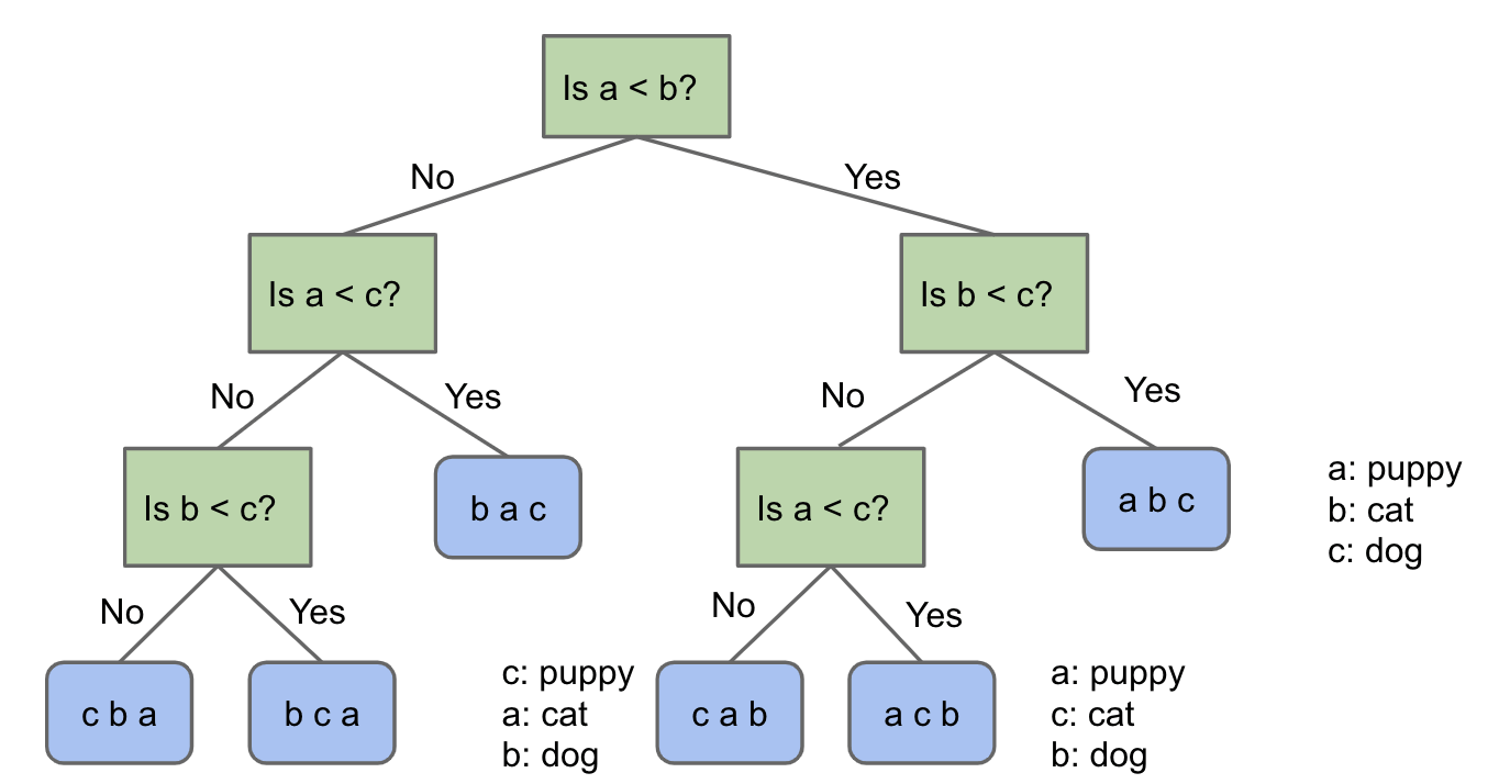
Game of Puppy, Cat, Dog

Suppose we have a puppy, a cat, and a dog, each in an opaque soundproof box labeled A, B, and C. We want to figure out which is which using a scale.

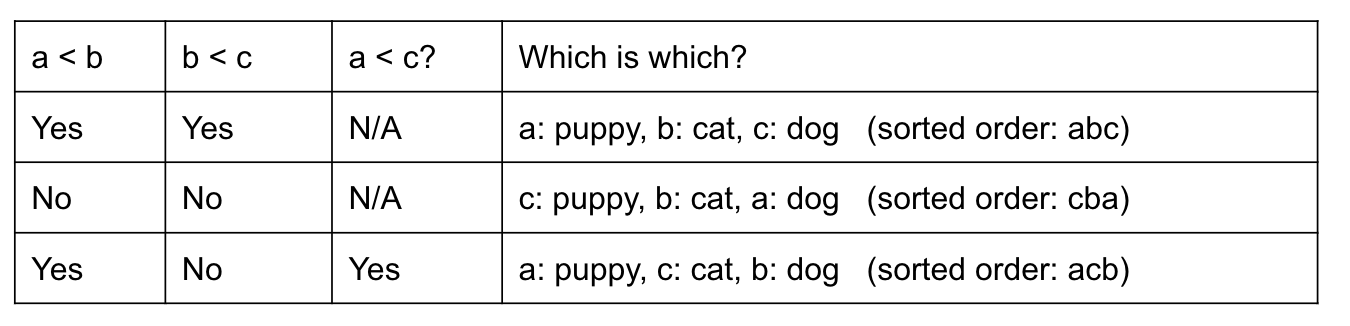
Notice that if we ask the first two questions a < b and b < c, and the answers are Yes and No, we can’t know the sorted order.

We can see the decision tree here:

How many questions would you need to ask to definitely solve the “puppy, cat, dog, walrus” problem?

The answer is 5.

• If $N = 4$, there are $4! = 24$ permutations.
• So we need a binary tree with 24 leaves.
  • How many levels minimum? $lg(24) = 4.58$, so 5 is the minimum. (some leaves are at level 6)

Let’s generalize the problem for $N$ items.

The answer is: $\Omega(\log{N!})$

• Decision tree needs $N!$ leaves.
• So we need $lg(N!)$ rounded up levels, which is $\Omega(\log{N!})$.

Generalization

Finding an optimal decision tree for the generalized version of this game is an open problem in mathematics.

Deriving a sequence of yes/no questions to identify these animals is hard, but we can use sorting to solve the problem.

In other words, this problem can reduce to sorting problem. Thus, any lower bound on difficulty of this game must also apply to sorting.

Since we have a lower bound on this game that it takes $\Omega(\log{(N!)})$ comparisons to solve such a puzzle in the worst case, sorting with comparisons also takes $\Omega(\log{(N!)})$ comparisons in the worst case.

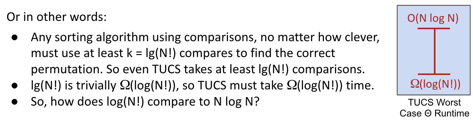
Since we have $\log{(N!)} \in \Omega(N\log{N})$, $\log{(N!)}$ grows at least quickly as $N\log{N}$, we can say the lower bound of TUCS is $\Omega(N\log{N})$.

Finally, any comparison based sort requires at least order $N\log{N}$ comparisons in its worst case.

Informally, we can say: TUCS >= Puppy, cat, dog >= $\log{(N!)}$ >= $N\log{N}$

Remember our goal is to try to bound the worst case runtime of sorting as close as possible.

Optimality

Note: In terms of sequential comparisons rather than parallel comparisons.

The punchline: Our best sorts have achieved absolute asymptotic optimality.

• Mathematically impossible to sort using fewer comparisons.
• Notice that randomized quicksort is only probabilistically optimal, but the probability is extremely high for even modest $N$. Are you worried about quantum teleportation? Then don’t worry about Quicksort.

Question: If we avoid comparing anything, can we do better in $\Theta(N)$ time?

Dodge The Bounds

We know that the ultimate comparison based sorting algorithm has a worst case runtime of $\Theta(N\log{N})$. But what if we don’t compare at all?

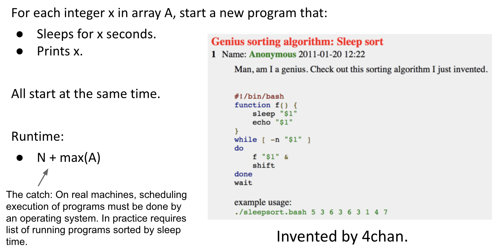
Sleep Sort

Example #1: Sleep Sort (for sorting integers, not good)

Counting Sort

Simplest Case

Example #2: Counting Sort (Exploiting Space Instead of Time)

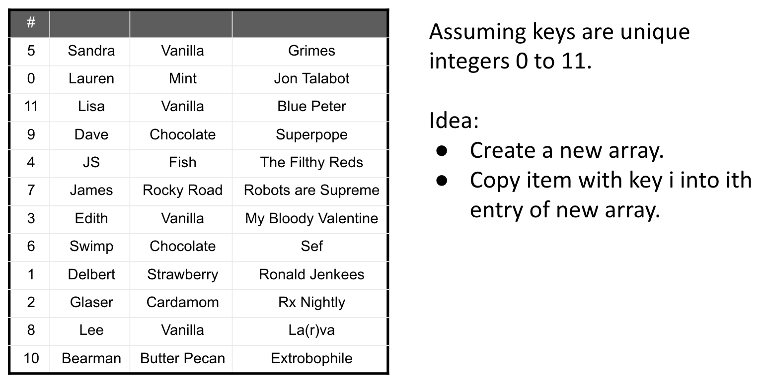
We just sorted $N$ items in $\Theta(N)$ worst case time, avoiding answer yes/no questions.

Simplest Case: Keys are unique integers from $0$ to $N-1$.

However, we may have some complex cases:

• Non-unique keys
• Non-consecutive keys
• Non-numerical keys

Alphabet Case

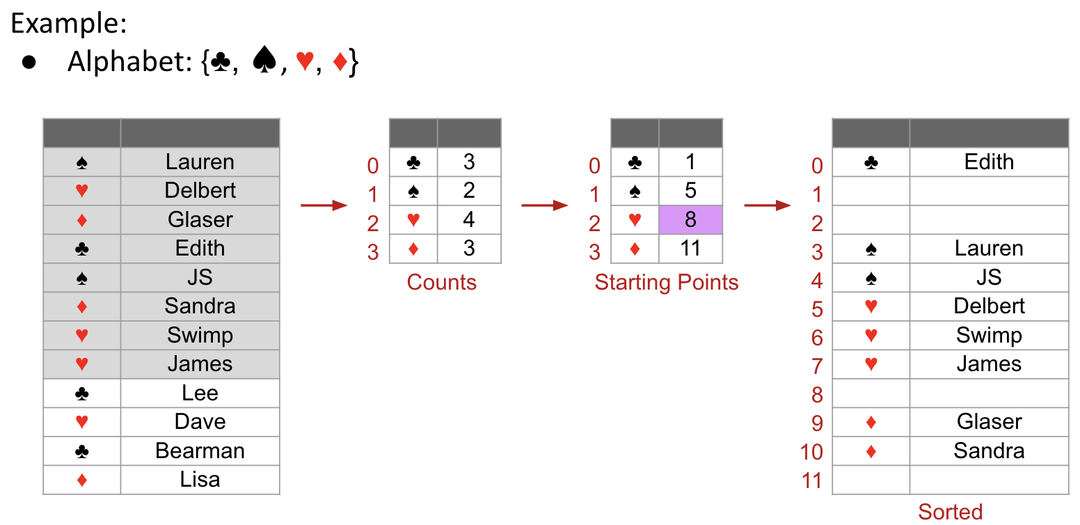
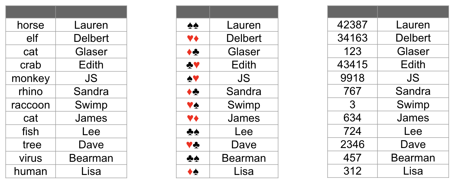
Alphabet Case: Keys belong to a finite ordered alphabet.

• Count number of occurrences of each item.
• Iterate through list, using count array to decide where to put everything.
• Based on the count array, initialize the starting point array.
• Iterate through list, guided by the starting point array to insert item into the sorted array, and update the starting point array.

Demo: link

Runtime

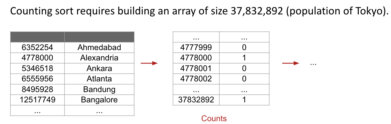
Question: For sorting an array of the 100 largest cities by population, which sort do you think has a better expected worst case runtime in seconds, Counting Sort or Quicksort?

The answer is Quicksort.

Question: What is the runtime for counting sort on $N$ keys with alphabet of size $R$?

Note: Treat $R$ as a variable, not a constant.

Runtime Analysis: Total runtime is $\Theta(N + R)$.

• Create an array of size $R$ to store counts: $\Theta(R)$
• Count number of each item: $\Theta(N)$
• Calculate target positions of each item: $\Theta(R)$
• Create an array of size $N$ to store ordered data: $\Theta(N)$
• Copy items from original array to ordered array, do $N$ times:
  • Check target position: $\Theta(1)$
  • Update target position: $\Theta(1)$
• Copy items from ordered array back to original array: $\Theta(N)$

Memory Usage: $\Theta(N + R)$

• $\Theta(N)$ is for ordered array.
• $\Theta(R)$ is for count and starting point arrays.

Bottom Line: If $N \geq R$, then we can expect reasonable performance.

So, if we want to sort really really big collections of items from some alphabet, counting sort is better.

Sort Summary (So Far):

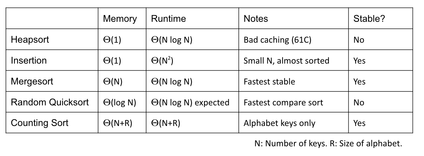
Note: Counting sort is nice, but alphabetic restriction limits usefulness. Also, it is not practical to store things like strings which have an infinite collection of keys.

Radix Sort

Although strings belong to an infinite collection of keys, they consist of characters from a finite alphabet.

LSD Radix Sort

LSD stands for Least Significant Digit, which is from rightmost digit towards left.

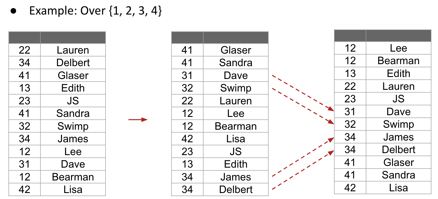
Note: The LSD is stable.

Runtime: $\Theta(WN + WR)$, where $W$ is the width fo .each item in # digits.

Non-Equal Key Lengths:

When keys are of different lengths, we can treat empty spaces as less than all other characters.

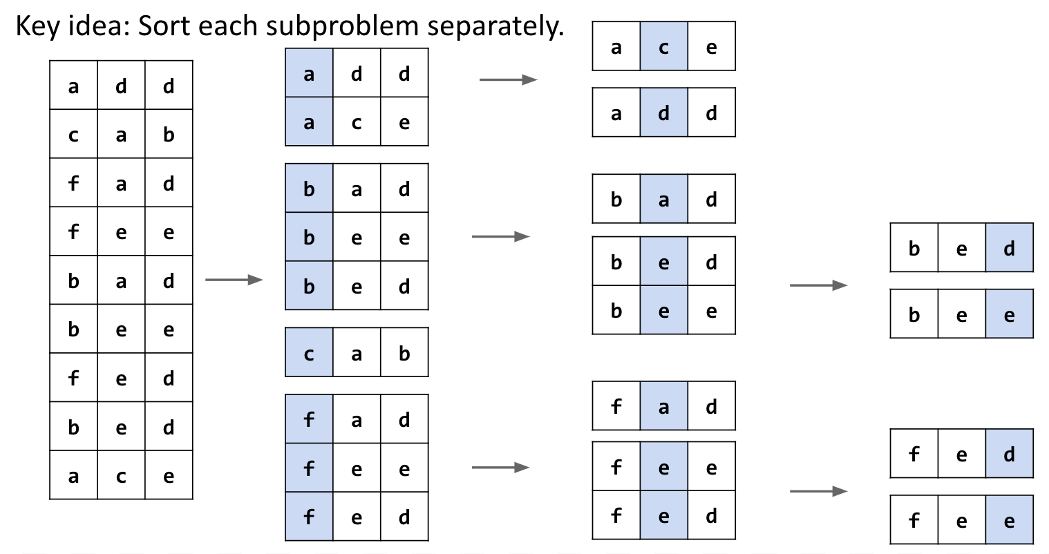
MSD Radix Sort

MSD stands for Most Significant Digit, which is from leftmost digit towards right.

Problem: If we treat MSD as what LSD did previously, it will end up a bad result.

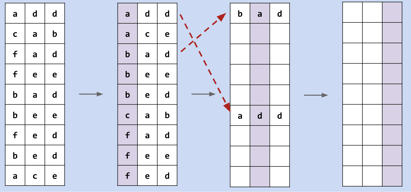
Solution: Sort each subproblem separately.

Runtime:

Best Case: We finish in one counting sort pass (the top digit is unique), looking only at the top digit: $\Theta(N + R)$.

Worst Case: We have to look at every character, degenerating to LSD sort: $\Theta(WN + WR)$.

Note: MSD has bad caching performance.

Sorting Runtime Summary:

Radix vs. Comparison

Intuitive Look

Question: Mergesort requires $\Theta(N\log{N})$ compares. What is Mergesort’s runtime on strings of length $W$?

It depends.

• $\Theta(N\log{N})$ if each comparison takes $\Theta(1)$ time.
  • Example: Strings are all different at the leftmost character.
• $\Theta(WN\log{N})$ if each comparison takes $\Theta(W)$ time.
  • Example: Strings are all equal.

LSD vs. Mergesort:

Assume that alphabet size is constant:

• LSD Sort has runtime $\Theta(WN + WR) = \Theta(WN)$.
• Mergesort has runtime between $\Theta(N\log{N})$ and $\Theta(WN\log{N})$.

Which one is better? It depends.

LSD is faster:

• Sufficiently large $N$.
  • $W$ is relatively small and we can treat it as a constant. Then LSD is linear and Mergesort is linearithmic.
• If strings are very similar to each other.
  • Each Mergesort comparison takes $\Theta(W)$ time.
    

Mergesort is faster:

• Strings are highly dissimilar from each other.
  • Each Mergesort comparison may finish early which costs constant time $\Theta(1)$.
    

Cost-Model Look

An alternate approach is to pick a cost model. Here we apply a cost model of character examination.

• Radix Sort: Calling charAt in order to count occurrences of each character.
• Mergesort: Calling charAt in order to compare two strings.

MSD vs. Mergesort:

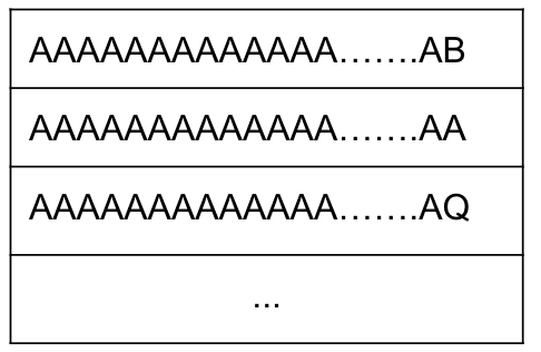
Suppose we have 100 equal strings of 1000 characters each. Estimate the total number of characters examined.:

• MSD:

  In the worst case (all strings are equal), every character is examined exactly once.

  So we have exactly $100 \times 1000 = 100,000$ total character examinations.

• Mergesort:

  Let’s first consider merge(100).

  Note: Merging 100 equal items results in always picking left.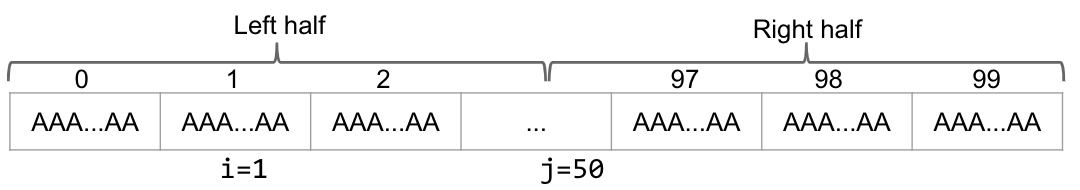

  

  • Comparing A[0] to A[50]: 2000 character examinations.
  • Comparing A[1] to A[50]: 2000 character examinations.
  • …
  • Comparing A[49] to A[50]: 2000 character examinations.
  • At last, the right half requires no comparison.
  • Total character examinations: $50 \times 2000 = 100,000$.

  So, merging $N$ strings of 1000 equal characters requires $1000N$ examinations.

  Since we have this recursive structure:

  

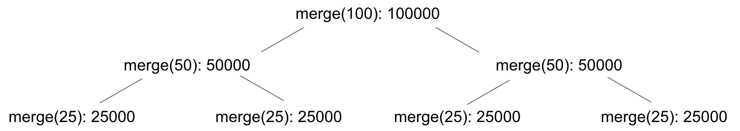
  $100000 + 50000 \times 2 + 25000 \times 4 + \ldots + merge(1) \times 100000 = ~660000$ characters.

  In total, we will examine approximately $1000N \times \log{N}$ characters.

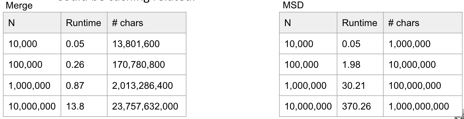
In summary, if character examinations are an appropriate cost model, we’d expect Mergesort to be slower by a factor of $\log{N}$. To see if we’re right, we’ll need to do a computational experiment.

Empirical Study

Computational experiment for $W = 100$.

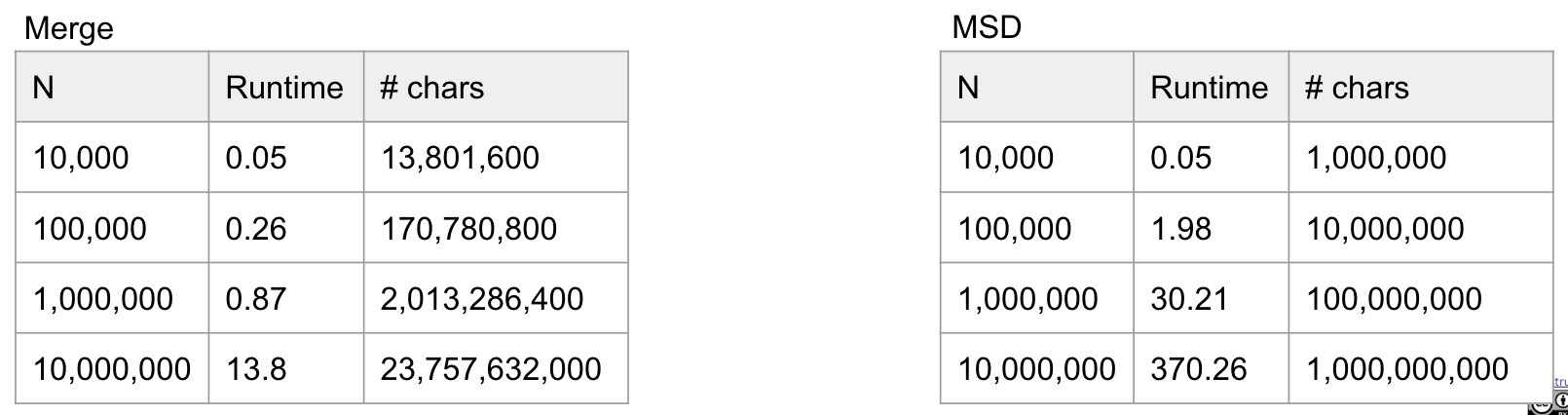
• MSD and Mergesort implementations are highly optimized versions.
• The data does not match our runtime hypothesis.
  • Our cost model isn’t representative of everything that is happening.
  • One particularly thorny issue: The Just-In-Time Compiler.

The Just-In-Time Compiler

Java’s Just-In-Time Compiler secretly optimizes your code when it runs, which means:

• The code you write is not necessarily the code will run.
• As code runs, the interpreter is watching everything that happens.
  • If some segment of code is called many times, the interpreter actually studies and re-implements your code based on what it learned by watching while running.

Example: The code below creates Linked List, 1000 at a time. Then repeat this 500 times yields an interesting result.

public class JITDemo1 {
  static final int NUM_LISTS = 1000;

  public static void main(String[] args) {
    for (int i = 0; i < 500; ++i) {
      long startTime = System.nanoTime();
      // Create 1000 linked lists
      for (int j = 0; j < NUM_LISTS; ++j) {
        LinkedList<Integer> L = new LinkedList<>();
      }
      long endTime = System.nanoTime();
      System.out.println(i + ": " + endTime - startTime);
    }
  }
}

• 1st Optimization: Not sure what it does.
• 2nd Optimization: Stops creating linked lists since we’re not actually using them.

Note: Add -Xint to VM options can discard the JIT feature.

Re-Run Experiments

Results with JIT disabled:

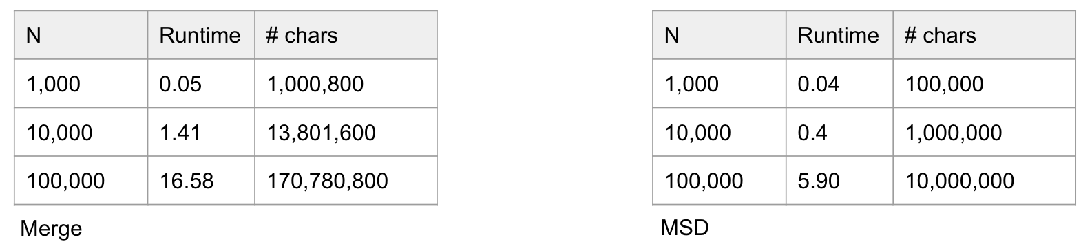
• Both sorts are much much slower than before.
• This time, Mergesort is slower than MSD (though not by as much as we predicted).

So, the JIT was somehow able to massively optimize the compareTo calls. It might know that comparing AAA...A to AAA...A over and over is redundant.

Also, the JIT seems to optimize Mergesort more than it does to MSD.

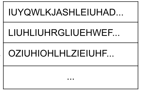
Plus, there are many possible cases to consider:

• Almost equal strings
• Randomized strings
• Real world data from some dataset of interest

Radix Sorting Integers

In the very large $N$ limit, Radix Sort is simply faster.

• Treat alphabet size as constant, LSD Sort has runtime $\Theta(WN)$.
• Comparison sorts have runtime $\Theta(N\log{N})$ in the worst case.

Issue: How do Radix Sort manage integer numbers?

• Option 1: Make them into a String. (Reduction Style)
• Option 2: Mods and floorMods and division operations to get the particular digit for integer. (faster and more general)

Note: Using the option 2, there’s no reason to stick with the base 10. We could instead treat as a base 16, 256, 65536 number.

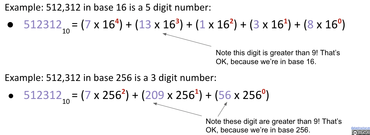
Runtime depends on the alphabet size.

• Size of the counting array $\Theta(R)$.
• Size of the width of the number $\Theta(W)$.

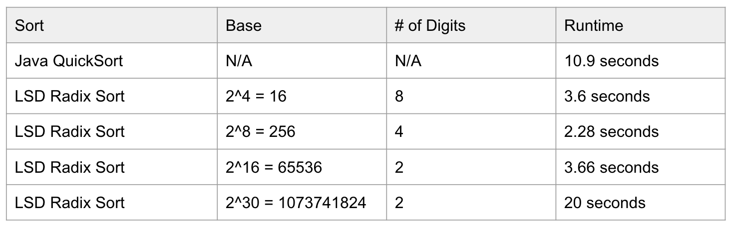
According to a computational experiment, a result of sorting 100,000,000 integers is as followed:

Sorting Summary

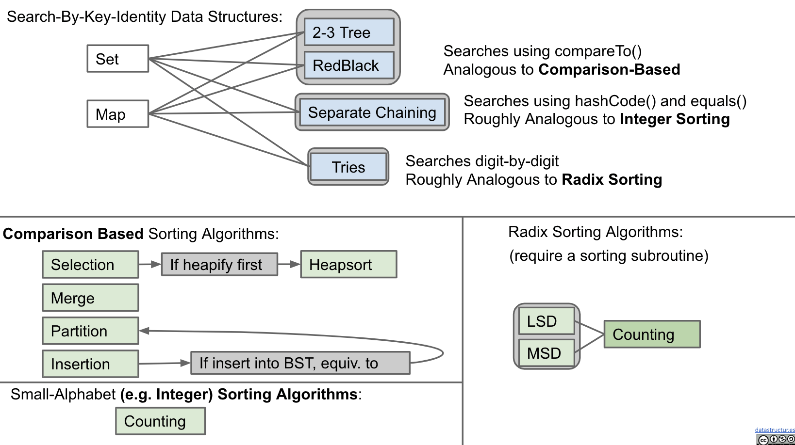
Three basic flavors: Comparison, Alphabet, and Radix based.

Each can be useful in different circumstances, but the important part was the analysis and the deep thought.

Sort vs. Search:

Search problem data structures:

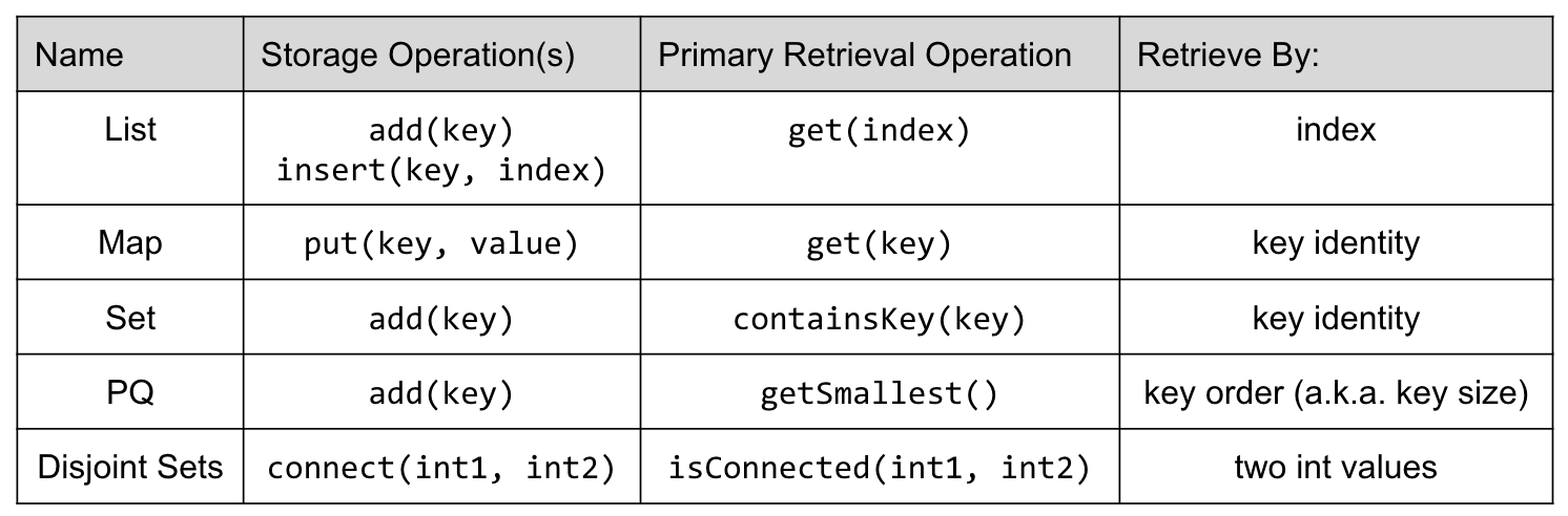
There are some interesting connections between sorting and searching (retrieval of interested data).

Connection:

Questions:

Ex (Guide)

Ex 1 (Which Sort?)

My Fall 2013 midterm, problem 7.

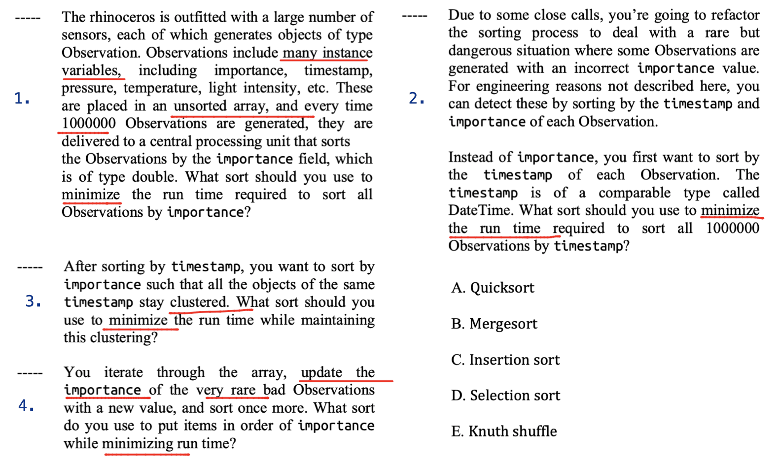
1. Quicksort. If we want to sort a set of randomly ordered items such that we get the best performance and don’t care about the stability, we should use Quicksort.
2. Quicksort or Insertion Sort. Don’t care about stability. Each of two is for randomly ordered or nearly sorted case.
3. Mergesort. We care about speed and stability this time. And the objects are randomly ordered.
4. Insertion Sort. Almost ordered.

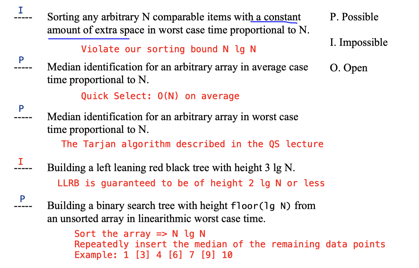
Ex 2 (Possible?)

Hug’s Spring 2013 midterm, problem 7.

Ex (Examprep)

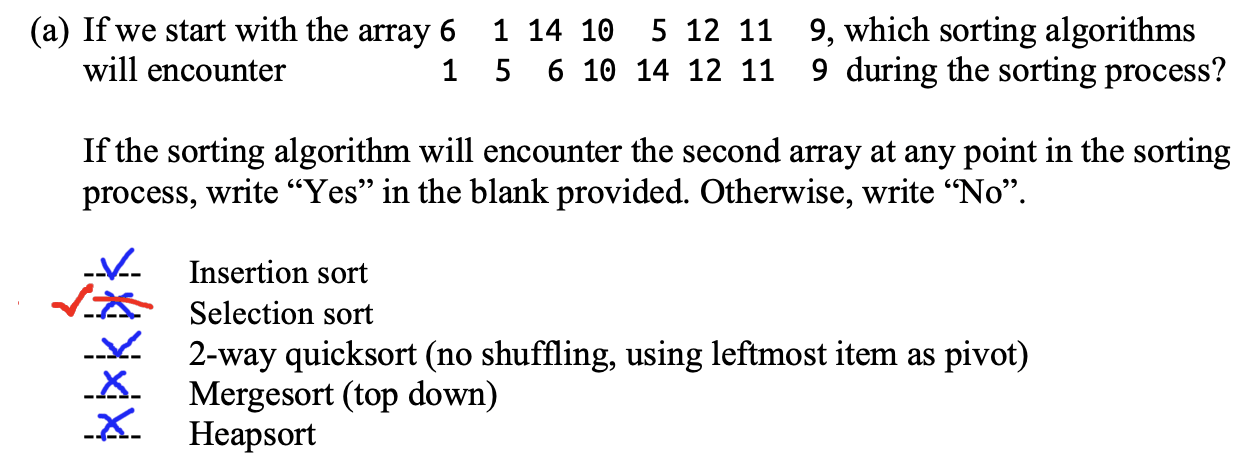
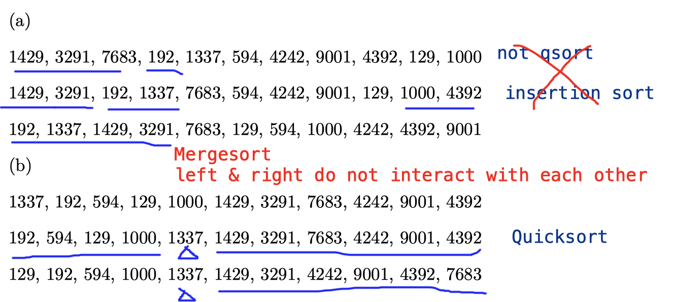
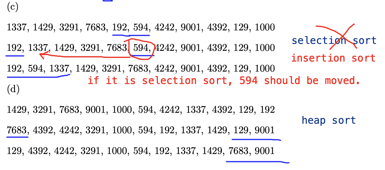
Ex 1 (Identifying Sorts)

Below you will find intermediate steps in performing various sorting algorithms on the same input list. The steps are not necessarily represent consecutive steps.

Choices: insertion sort, selection sort, mergesort, quicksort (first element as pivot), and heapsort.

Input list: 1429, 3291, 7683, 1337, 192, 594, 4242, 9001, 4392, 129, 1000

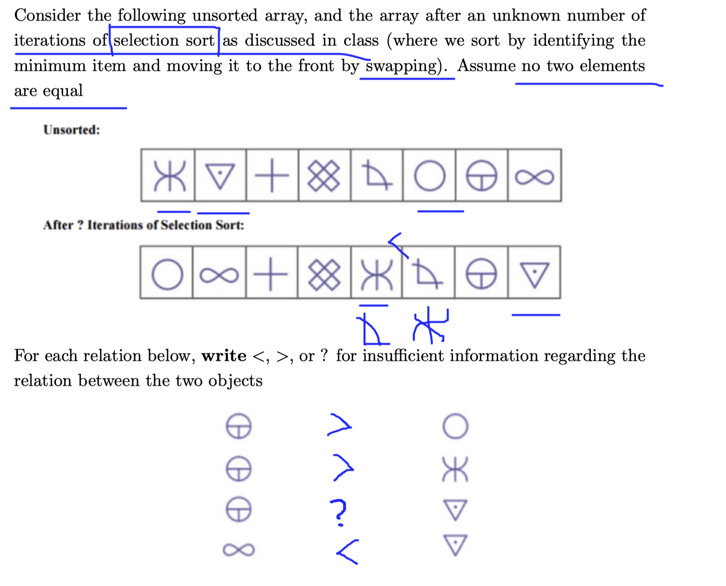
Ex 2 (Reverse Engineering)

Ex 3 (Conceptual Sorts)

Choices:

A. Quicksort
B. Mergesort
C. Selection Sort
D. Insertion Sort
E. Heapsort
N. (None of the above)

• A B E: Bounded by $\Omega(N\log{N})$ lower bound.
• B E: Has a worst case runtime that is asymptotically better than Quicksort’s worstcase runtime.
• C: In the worst case, performs $\Theta(N)$ pairwise swaps of elements.
• A B D: Never compares the same two elements twice.
• N: Runs in the best case $\Theta(\log{N})$ time for certain inputs.

Ex 4 (Quickselect)

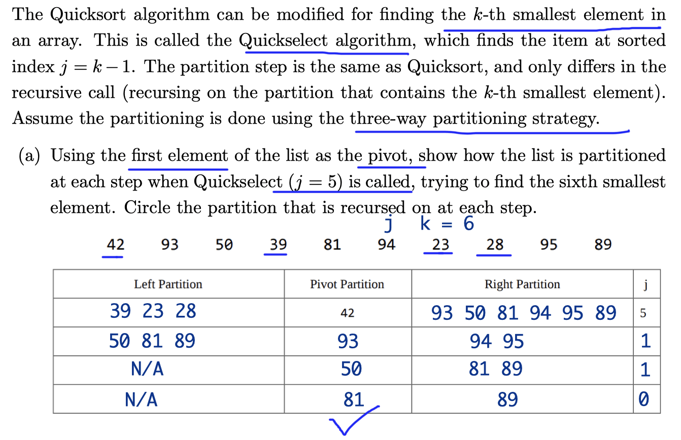
(b) What is the best and worst case runtime of Quickselect?

Best: $O(N)$, the first pivot is the one we want.
Worst: $O(N^2)$

(c) Assume we use Quickselect to find the median of an array and always choose the median as the pivot. In this case, what would be the best and worst case runtime of Quicksort?

Best: $O(N\log{N})$
Worst: $O(N^2)$

• Quickselect in worst case: $O(N^2)$
• Quicksort now in best case: $O(N\log{N})$

Ex 5 (Radix Sorts)

Marked

Answer: M

Ex 7 (N is large)

Note: $N$ is very large.

Choosing from among:

1. Insertion Sort
2. Mergesort
3. Quicksort (with Hoare Partitioning)
4. LSD Radix Sort

No. 2 and 5 are marked.

Ex 8 (Monotonically Improving)

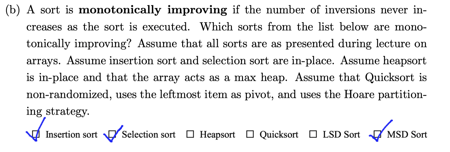
Heapsort and Quicksort are marked.