CS 61B | Part 10 | Shortest Paths (SP), Minimum Spanning Trees (MST)

Shortest Paths

BFS vs. DFS for Path Finding

Possible consideration:

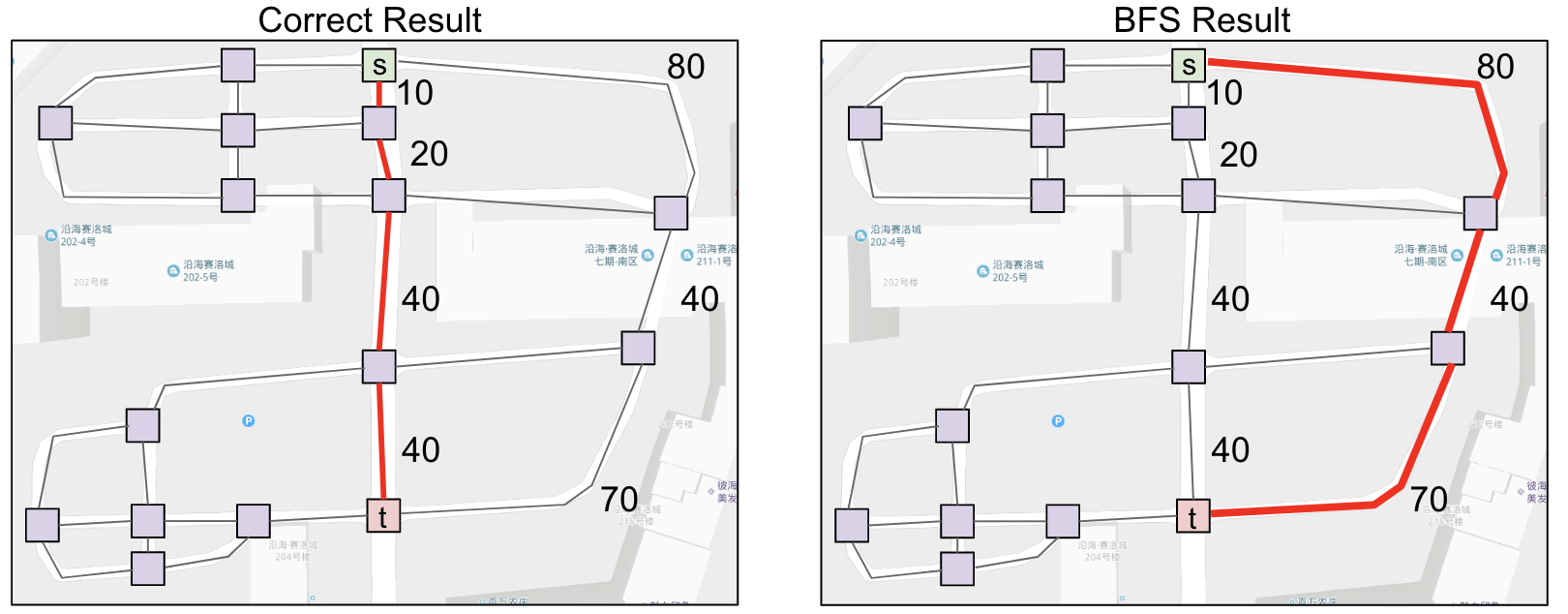
• Correctness. Do both work for all graphs?
• Output Quality. Does one give better results?
  • BFS is a 2-for-1 deal, not only do you get paths, but your paths are also guaranteed to be shortest.
• Time Efficiency. Is one more efficient than the other?
  • Should be very similar. Both consider all edges twice.

What about space efficiency?

• DFS is worse for spindly graphs.
  • Call stack gets very deep. Need $\Theta(V)$ memory to remember recursive calls.
• BFS is worse for absurdly bushy graphs.
  • Queue gets very large. In worst case, queue will require $\Theta(V)$ memory. For example, one vertex connects with the rest of 1,000,000 vertices.

Note: In our implementation, we have to spend $\Theta(V)$ memory anyway to track distTo and edgeTo arrays. But we can optimize by storing in a map.

But BFS has a problem. It returns a path with shortest number of edges.

By Eyes

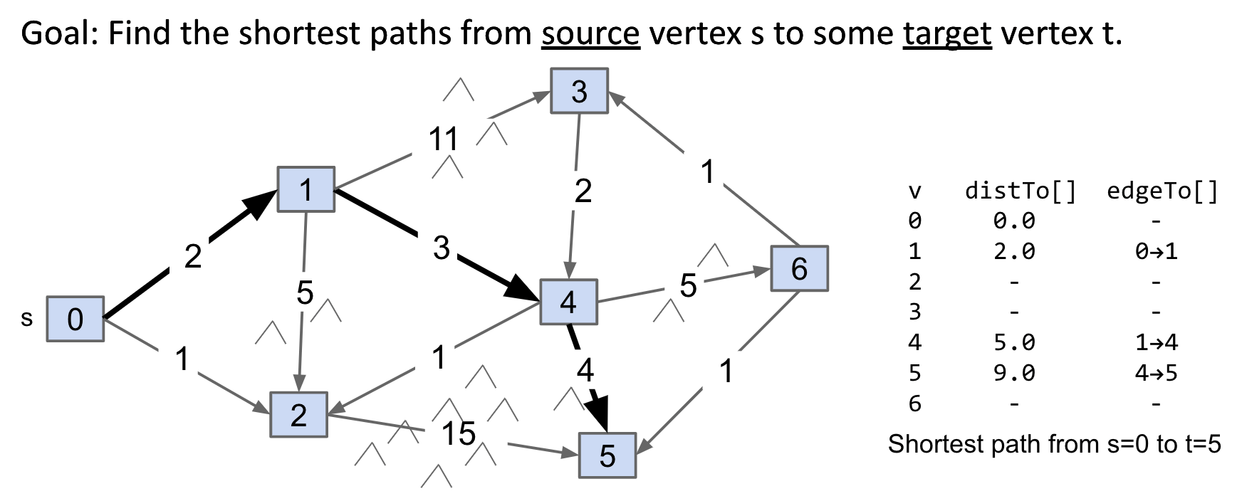
Observation: Solution will always be a path with no cycles (assuming non-negative weights).

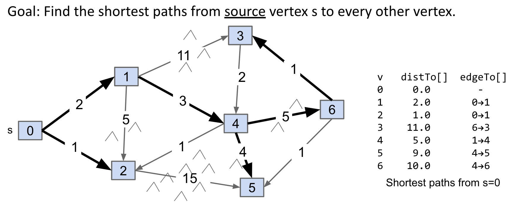
Observation: Solution will always be a tree (a union of all the shortest paths to all vertices).

Note: All still hold for undirected graphs.

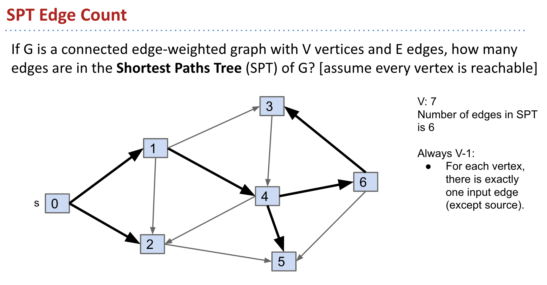
The number of edges in the tree is always $V - 1$.

$D_{in}$ is always equal to $1$.

Bad Algorithms

Bad Algorithm #1:

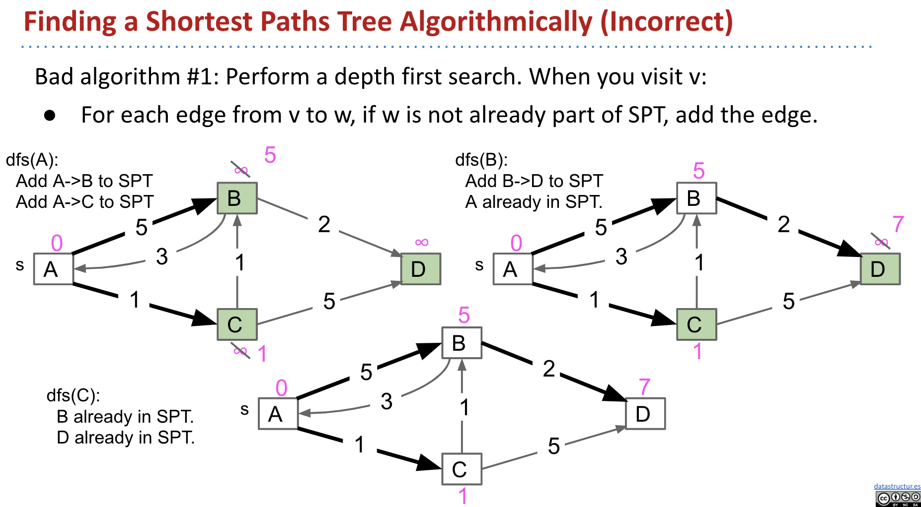
In dfs(C), we don’t update the edge C->B anymore.

Bad Algorithm #2:

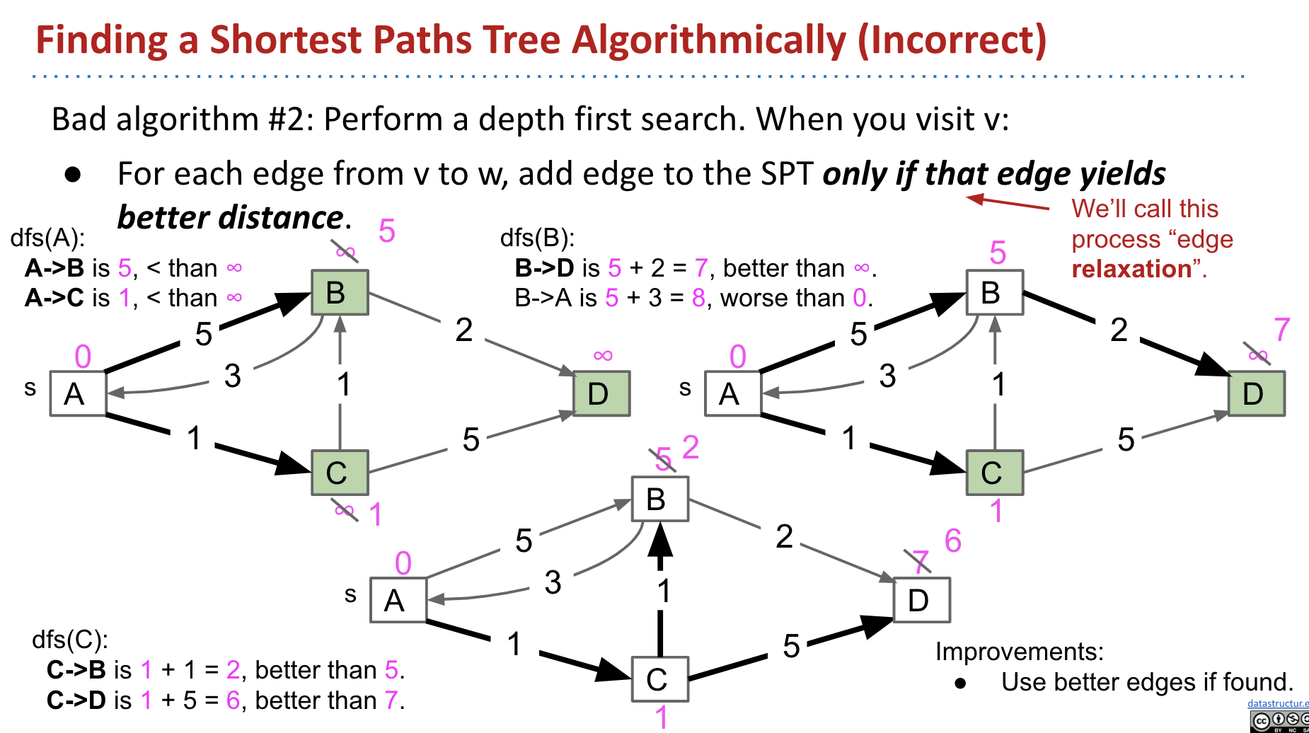
Why? We’ve updated B, but not updated the value $7$ in D.

We can go back to B and dfs(B) again, but it’s slower.

The problem lies in the fact that we visit B first and then C. If we visit C first, the problem no long exists.

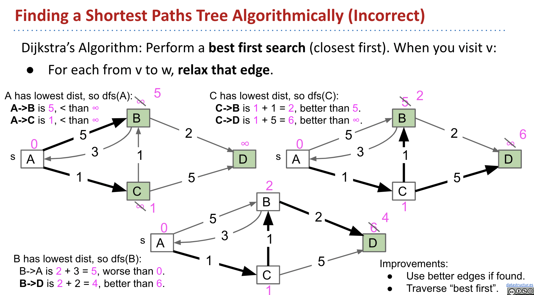
Dijkstra’s Algorithm

Basic Idea

Error: Should not be dfs().

You should write it by hands and by yourself!

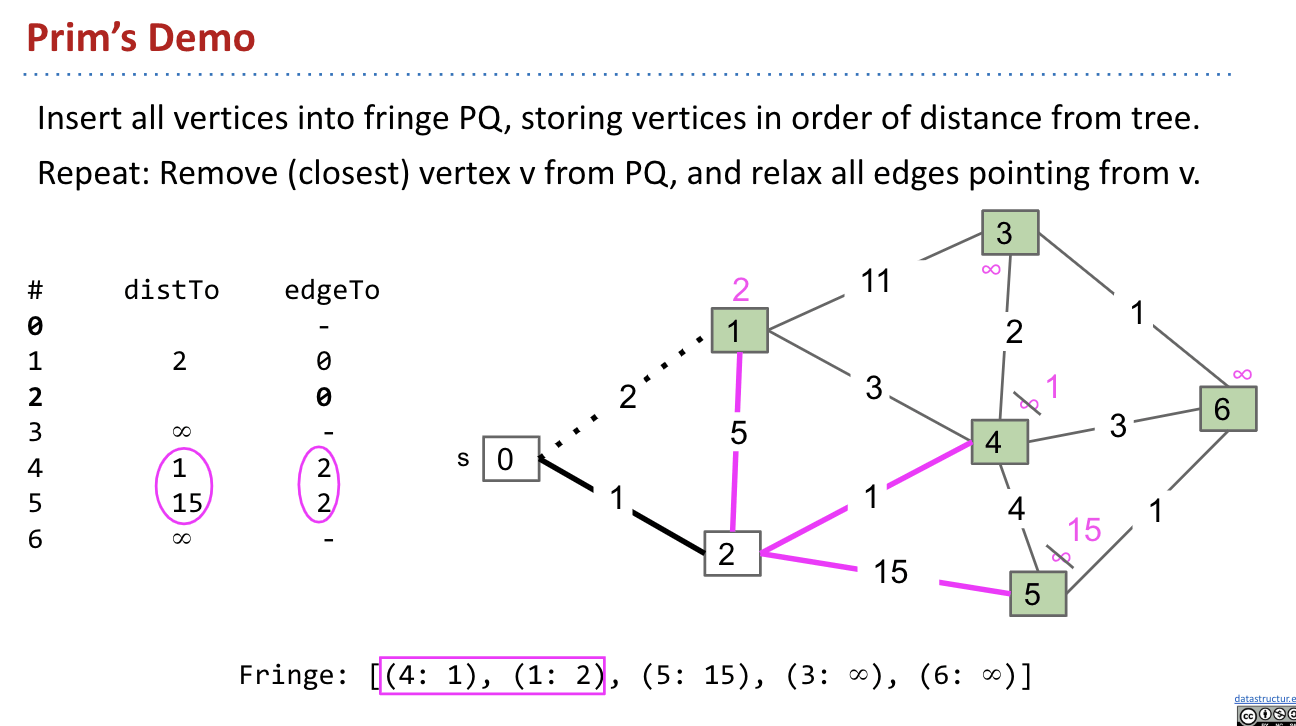
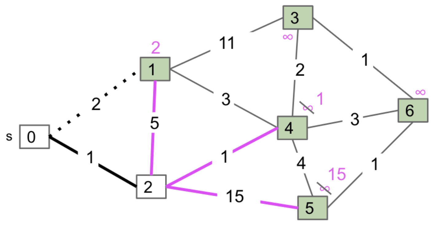
Dijkstra’s Algorithm: Perform a best first search (closest first).

We use a Fringe (Priority Queue) to keep track of which vertex is closest to the source.

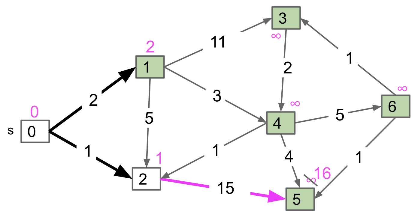
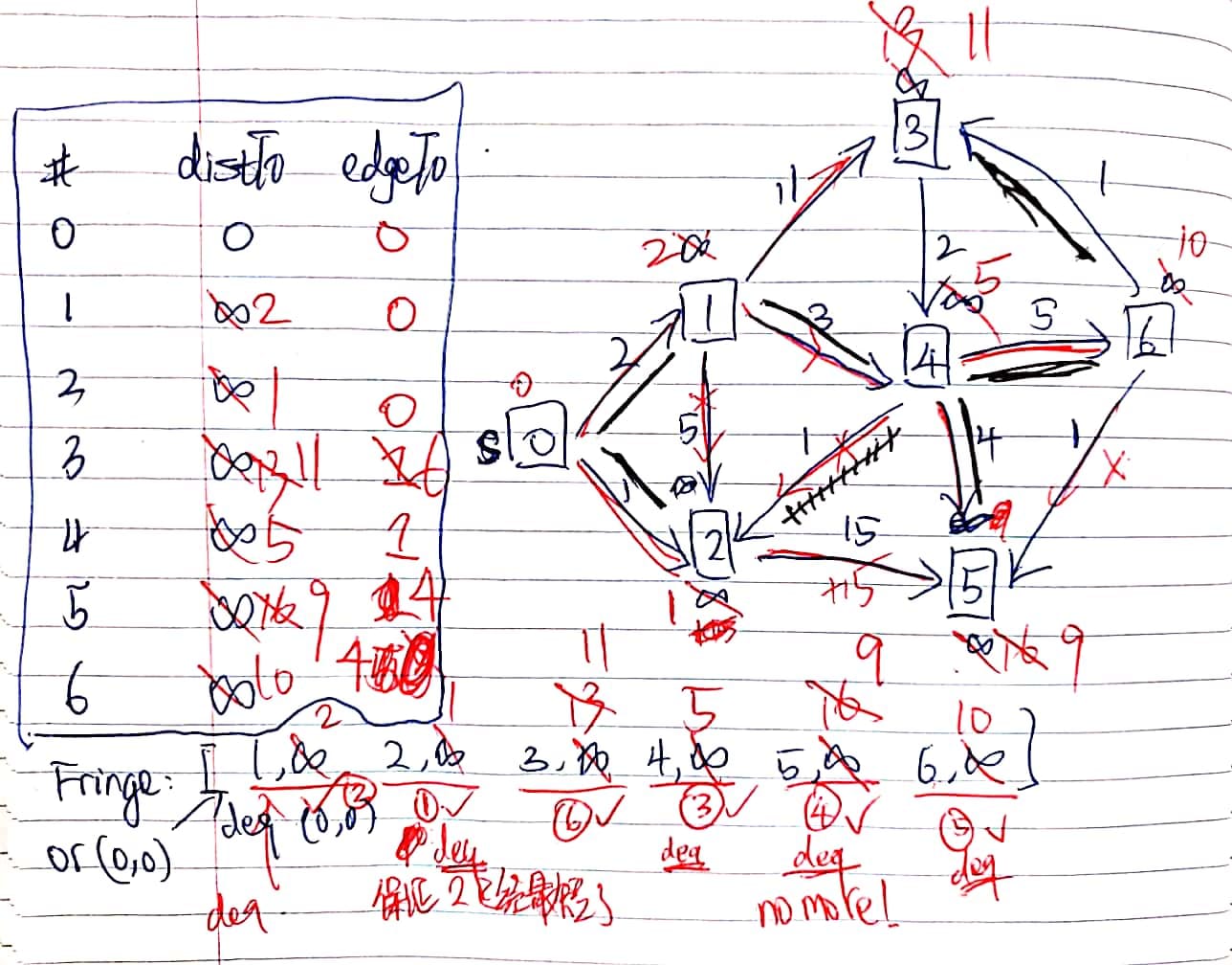
Walkthrough

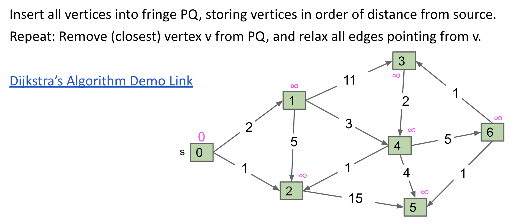
Demo: link

You should write it by hands and by yourself!

Every time we start looking more vertices from the vertex that is closest to the source. This is the reason why we use the priority queue Fringe to keep track of the vertex we want.

When doing dequeue(), we can assure that the path from the source to this vertex is already the shortest! Why?

There is a premise that weights could not be negative. Therefore, it is impossible that a future path that is back to, for example vertex 2, must be at least greater than $1$.

Note: Also, notice that when dequeueing vertex 1, there is no potential shortest path from vertex 2 to vertex 1 (we have checked). If there was, I would have updated the value of vertex 1.

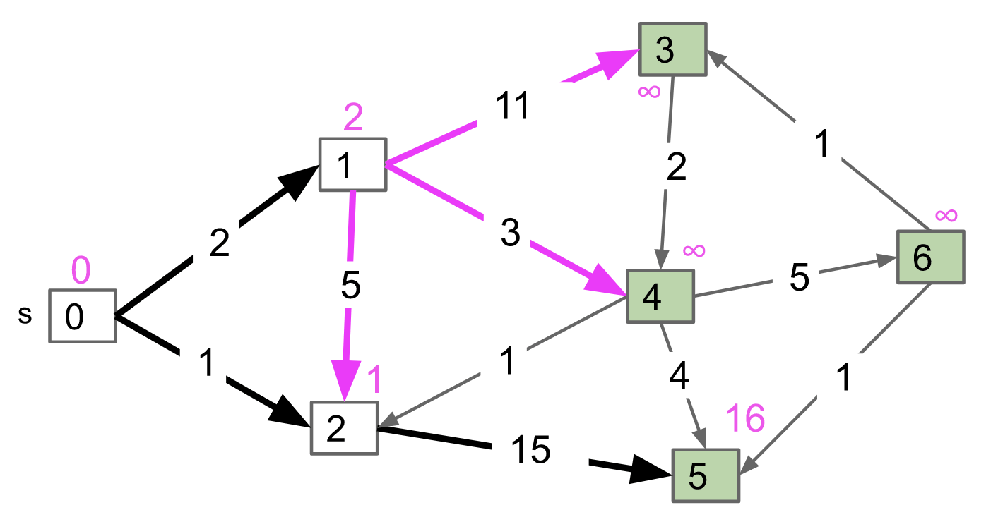
After dequeueing vertex 1, we examine vertex 2, 3, 4. As for vertex 2, do we need to update its value? No! We don’t even go to it. Because we’ve already said distTo[2] has been finalized (vertex 2 has been dequeued before). No more potential update for vertex 2. (only for non-negative weights)

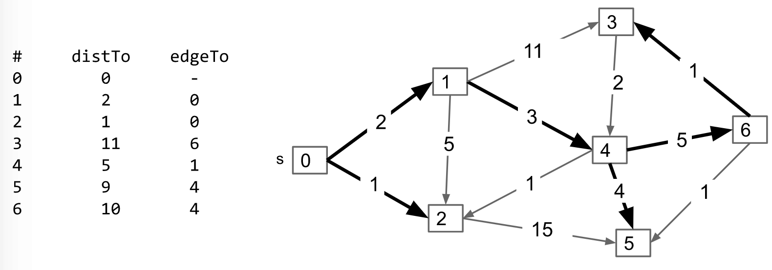
Finally, we have:

Key Properties

One-sentence Idea:

Visit vertices in order of best-known distance from source. On visit, relax every edge from the visited vertex to unvisited vertices.

Key Invariants:

• edgeTo[v] is the best known predecessor of $v$.
• distTo[v] is the best known total distance from source to $v$.
• PQ contains all unvisited vertices in order of distTo[].

Important properties:

• Always visits vertices in order of total distance from the source.
• Relaxation always fails on edges to visited vertices (white, not in the queue).
  • Because it always makes that worse.

Guaranteed Optimality:

The Idea of “Suppose that it isn’t the case.”
The Idea of “Proof by Induction.”

Dijkstra’s is guaranteed to be optimal so long as there are no negative edges.

• Proof relies on the property that relaxation always fails on edges to visited vertices.

Premise: Assume all edges have non-negative weights.

Proof by Induction: Relaxation always fails on edges to visited vertices.

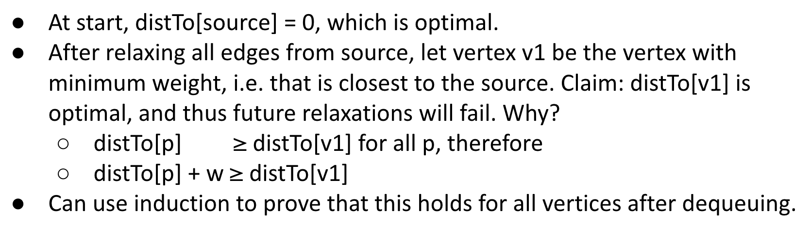
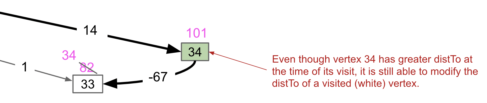
So, if $w$ is a negative number, this property no longer holds because distTo[p] + w might be less than distTo[v1]. Relaxation of already visited vertices can succeed as follows.

Try this out:

Suppose that your graph has negative edges, but all the negative edges only go out of the source vertex $s$ that you were passed in. Does Dijkstra’s work? Why / Why not?

Still work. When the 1-level vertex is dequeued, the shortest distance is finalized, although it has a negative value. Since later weights are all non-negative, it’s impossibly necessary to relax the node.

How to deal with negative weights?

• No cycles. BFS the tree to relax.
• Cycles exist. Bellman-ford: For every vertex, relax all the edges. => $O(V)$

Short-circuiting

One nice consequence of this fact is short-circuiting. Suppose that you wanted to take, like, the cities of the world on a graph, and find the shortest path from Berkeley to Oakland. Running dijkstra(Berkeley) will mean that you can’t actually stop this powerful beast of an algorithm. Once Oakland is popped off the priority queue in the algorithm, we can just stop. So sometimes dijkstra’s takes in not only a source, but also a target.

Pseudocode

Note: In the version in class, we did not use an explicit mark. Instead, we tossed everything in the PQ, and we effectively considered a vertex marked if it had been removed from the PQ.

Dijkstra’s:

• PQ.add(source, 0)
• For other vertices $v$, PQ.add(v, Infinity)
• While PQ is not empty:
  • p = PQ.removeSmallest()
  • Relax all edges from $p$

Relaxing an edge $p$ -> $q$ with weight $w$:

• If $q$ is popped (i.e., $q$ is not in PQ):
  • continue
• If distTo[p] + w < distTo[q]:
  • distTo[q] = distTo[p] + w
  • edgeTo[q] = p
  • PQ.changePriority(q, distTo[q]) // O(log V)

Runtime Analysis

Priority Queue operation count, assuming binary heap based PQ:

• add: $V$ times, each costing $O(\log{V})$ time.
• removeSmallest: $V$ times, each costing $O(\log{V})$ time.
• changePriority: $E$ times, each costing $O(\log{V})$ time. (in other words, $E$ times relaxing in the worst case)

So the overall runtime is $O(V\log{V} + V\log{V} + E\log{V}) = O((V + E)\log{V})$.

Assuming $E > V$, this is just $O(E\log{V})$ for a connected graph.

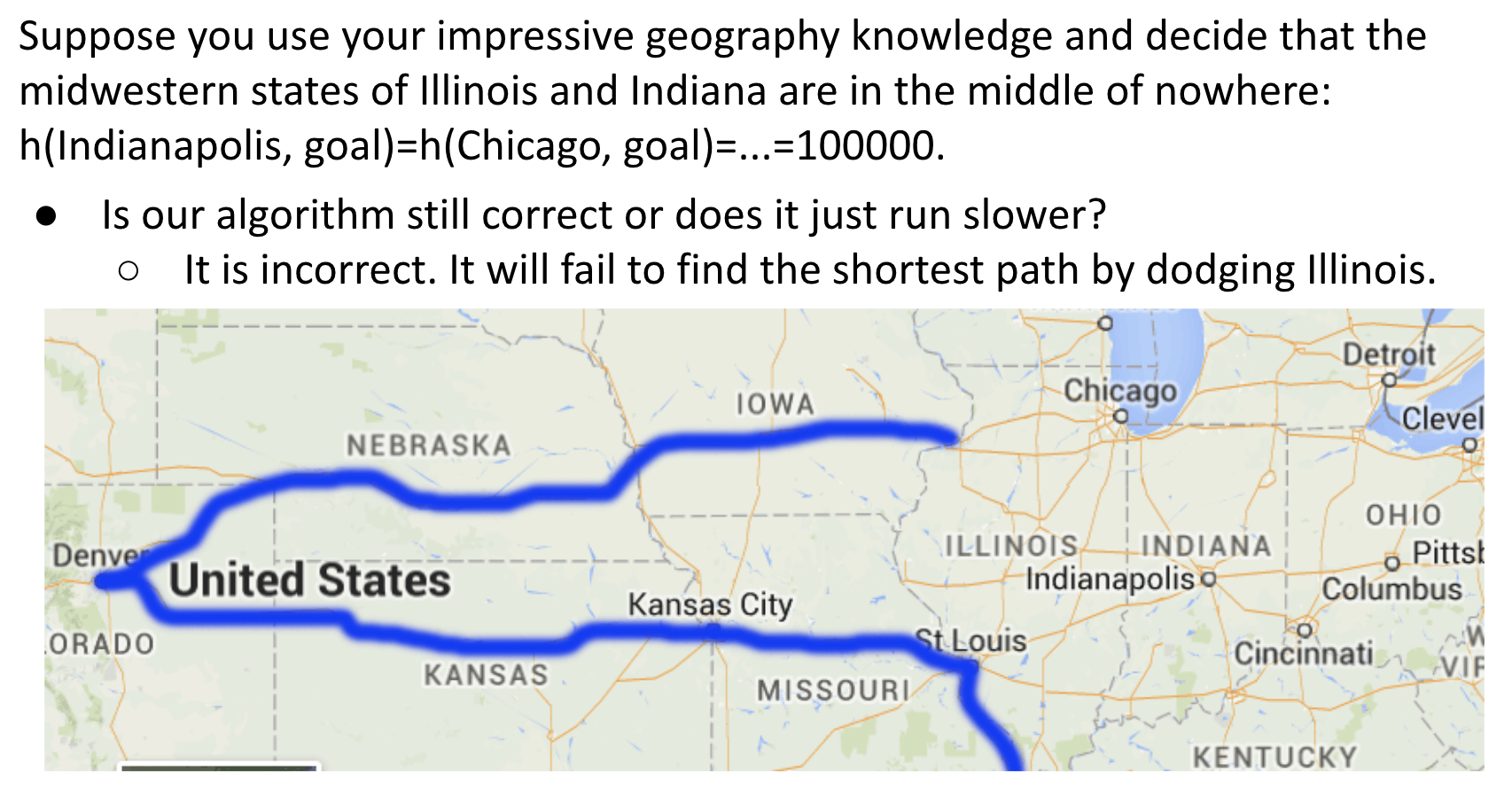
A* Algorithm

The Problem with Dijkstra’s:

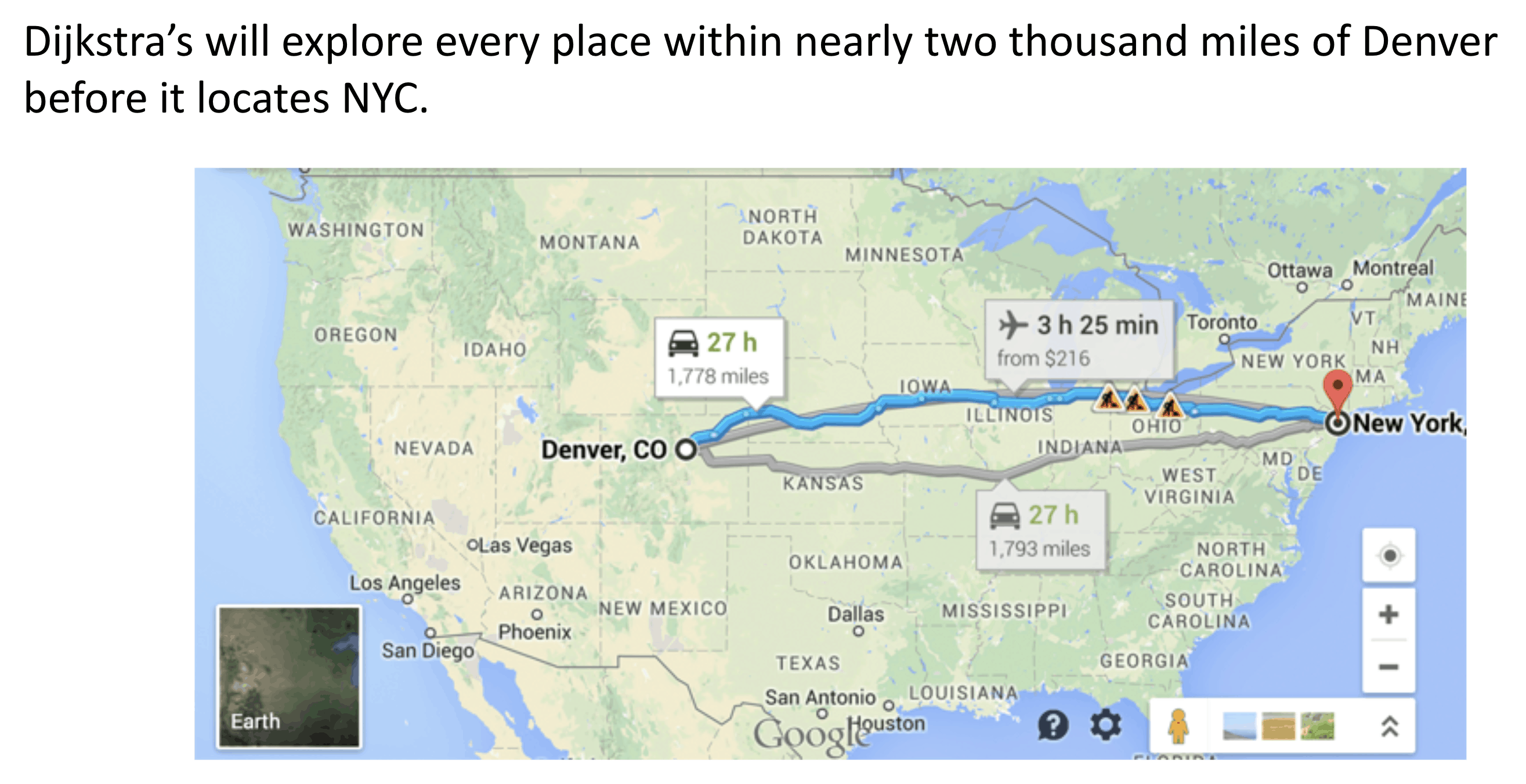
It’ll end up traversing nodes in closest concentric circle order.

We have only a single target in mind, so we need a different algorithm.

Simple Idea:

• Visit vertices in order of d(Denver, v) + h(v, goal), where h(v, goal) is an estimate of the distance from $v$ to our goal NYC.
• In other words, look at some location $v$ if:
  • We already know the fastest way to reach $v$.
  • AND we suspect that $v$ is also the fastest way to NYC taking into account the time to get to $v$.

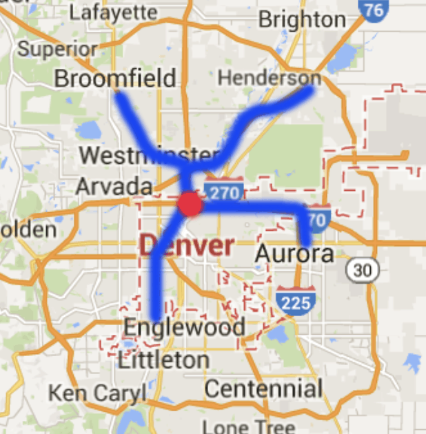
Example: Henderson is farther than Englewood, but probably overall better for getting to NYC.

A* Demo: link

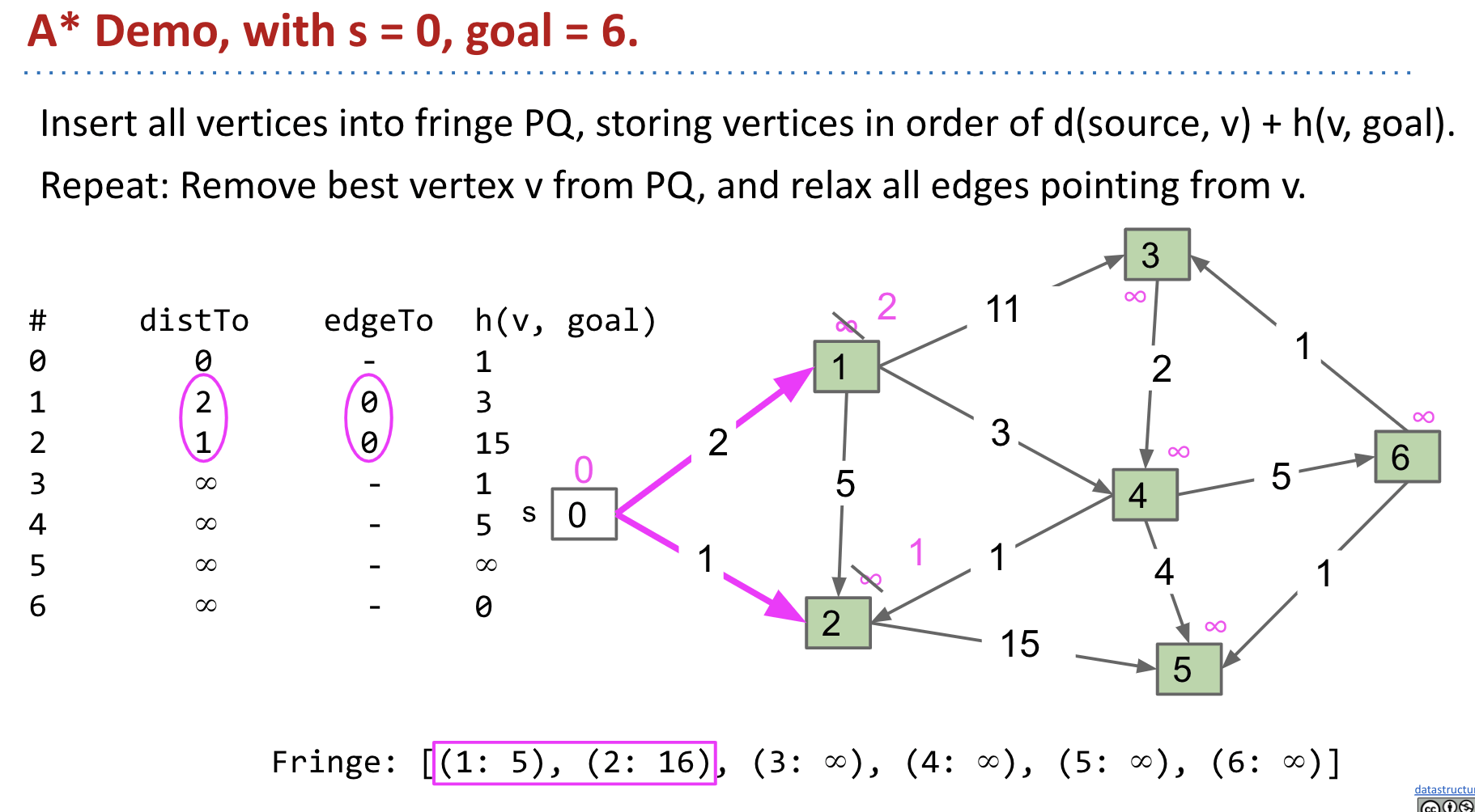
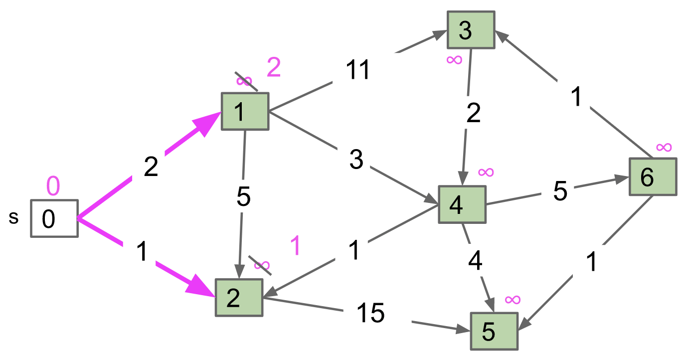
This time we go to vertex 1 instead of 2 because $2 + 3 < 1 + 15$.

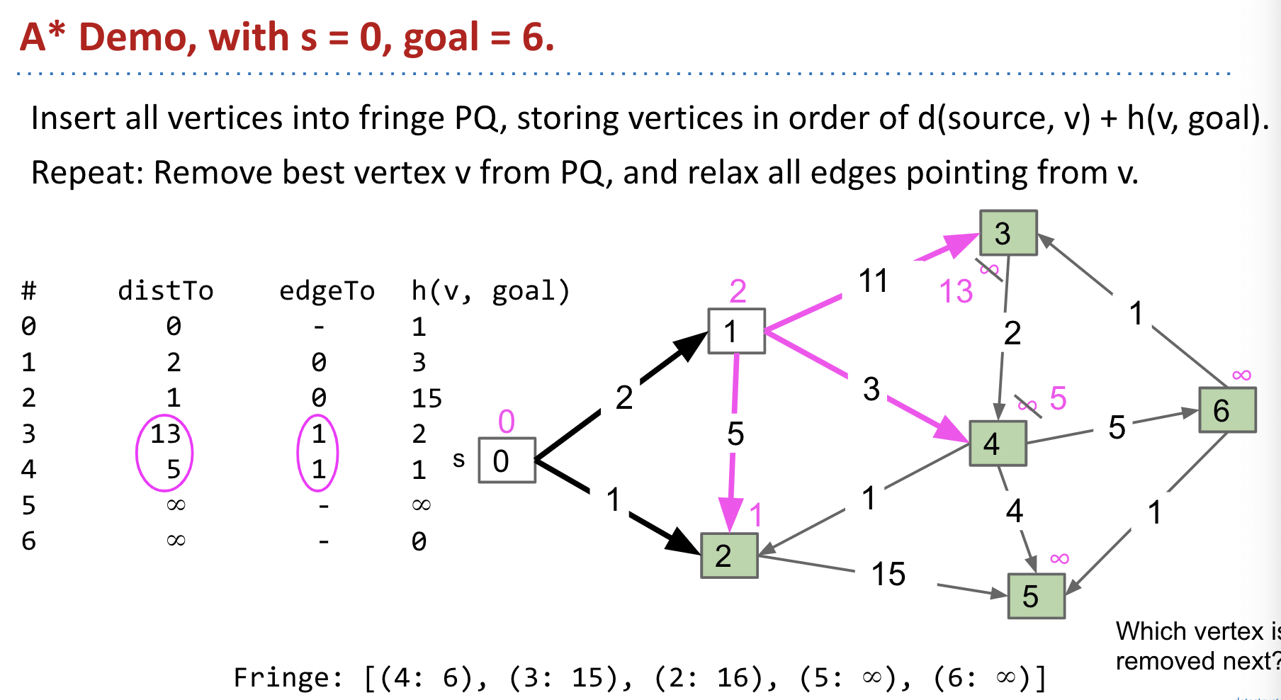
Then we go to vertex 4 because $4 + 1 = 5$ is minimum (vertex 2: $1 + 15 = 16$, vertex 3: $13 + 2 = 15$).

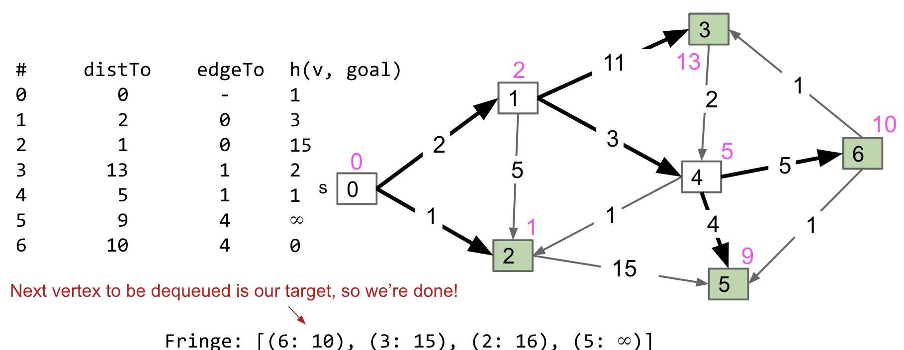
Finally, go to vertex 6. Go over the last operations (check vertex 3 and 5) and then dequeue it.

Observations:

• Not every vertex got visited.
• Result is not a shortest paths tree for vertex 0, since path to vertex 3 is suboptimal! But it’s OK because we only care about the path to vertex 6, our goal.

Impact of Heuristic Quality:

For our version of A* to give the correct answer, our A* heuristic must be:

• Admissible: $h(v, NYC) \leq$ true distance from $v$ to $NYC$.
  • Never overestimates.
• Consistent: For each neighbor of $w$:
  • $h(v, NYC) <= dist(v, w) + h(w, NYC)$
  • Where $dist(v,w)$ is the weight of the edge from $v$ to $w$.

Simply know that choice of heuristic matters, and that if you make a bad choice, A* can give the wrong answer.

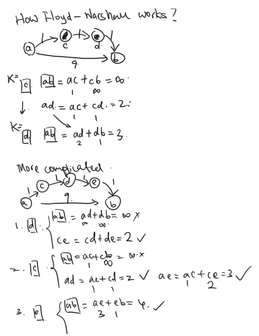
Floyd-Warshall

Floyd-Warshall All Pairs Shortest Path Algorithm (APSP) | Graph Theory

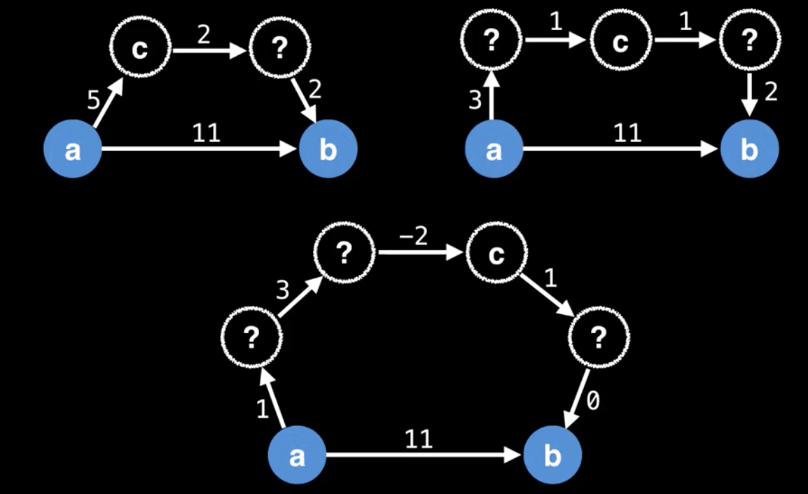
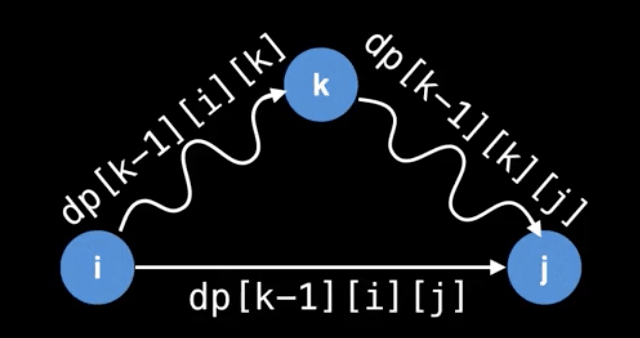
Main Idea: Gradually build up all intermediate routes between nodes $i$ and $j$ to find the optimal path.

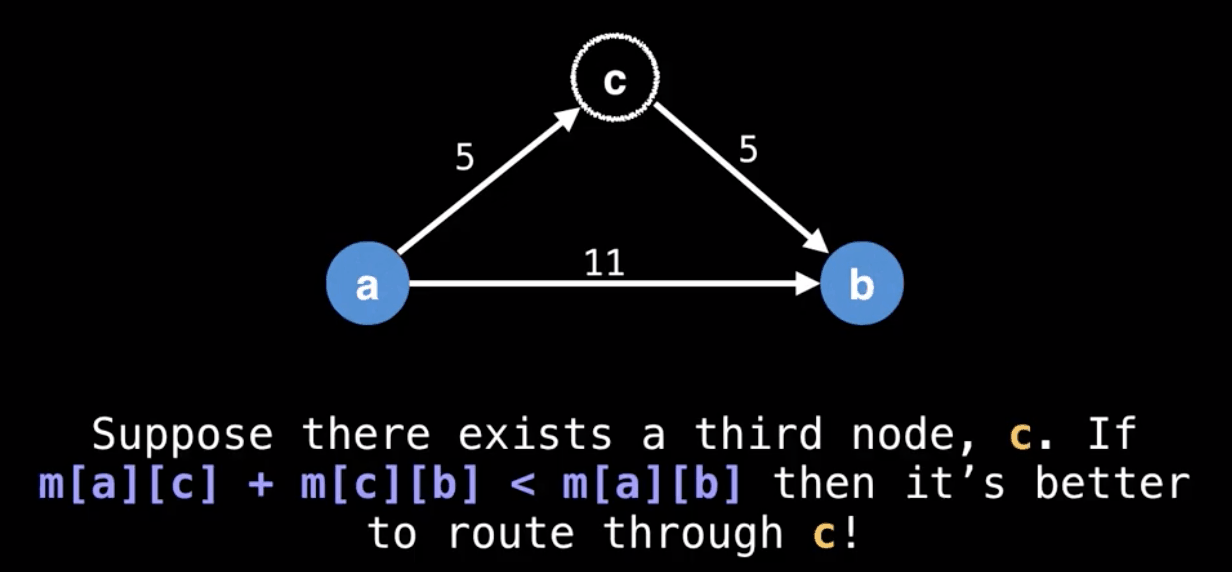
The goal of Floyd-Warshall is to eventually consider going through all possible intermediate nodes on paths of different lengths.

In the beginning the optimal solution from $i$ to $j$ is simply the distance in the adjacency matrix.

$$dp[k][i][j] = m[i][j],\ \text{if}\ k = 0$$

otherwise:

$$dp[k][i][j] = min(dp[k -1][i][j], dp[k-1][i][k] + dp[k-1][k][j])$$

In terms of memory usage, it is possible to compute the solution for k in-place saving us a dimension of memory and reducing the space complexity to $O(V^2)$.

The new recurrence relation is:

$$d[i][j] = m[i][j], \ \text{if}\ k = 0$$

otherwise:

$$dp[i][j] = min(dp[i][j], dp[i][k] + dp[k][j])$$

Ex (Guide)

C level

Ex 1 (pathTo)

Implement public Iterable<int> pathTo(int w) method that returns an Iterable of vertices along the path:

private int[] edgeTo;
private int[] distTo;

public int distTo(int w) {
  return distTo[w];
}

public Iterable<Integer> pathTo(int w) {
  List<Integer> path = new LinkedList<>();
  pathTo(w, path);
  return path;
}

// edgeTo[0] = 0
private void pathTo(int w, List<Integer> path) {
  path.addFirst(w);
  if (w == 0) {
    return;
  }
  pathTo(edgeTo[w], path);
}

Ex 2 (SP Practice)

Problem 4 from Princeton’s Fall 2009 final.

Very trick. Need to be very careful when handling with the last nodes.

Ex 3 (Add A Constant)

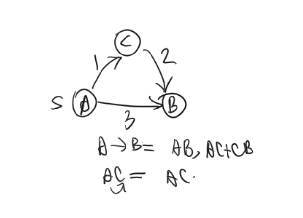
True or false: Adding a positive constant $k$ to every edge weight does not change the solution to the single-source shortest-paths problem.

False. Adding a constant to all the edge weights when calculating shortest paths means we start favoring paths that use fewer edges. As a concrete example:

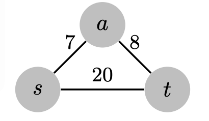
Start from $s$.

Ex 4 (Multiply A Constant)

True or false: Multiplying a positive constant to every edge weight does not change the solution to the single-source shortest-paths problem.

True. No accretion effect.

Ex 5 (A* Practice)

Problem 9 from my Spring 2015 final.

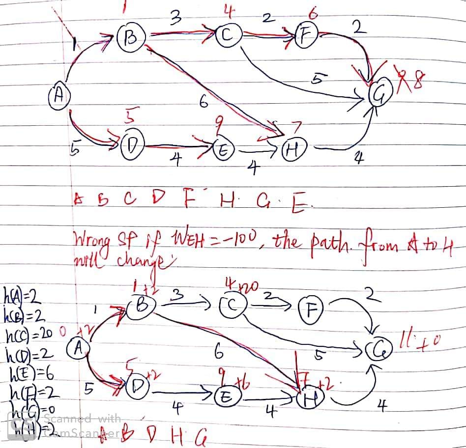
We see h(C) = 20, but the actual cost to $G$ is $4$, so the heuristic is not admissible, and A* is not guaranteed to return the correct SP (A-B-C-F-G).

So SP to $G$ (A*): A-B-H-G.

B level

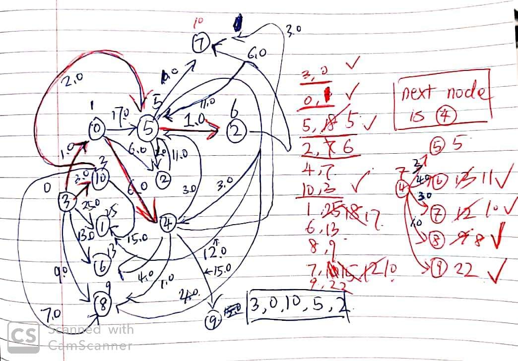
Ex 1 (Deduction)

Great problem.

Problem 4 from Princeton’s Fall 2011 final. Note that when the exam says to “relax a vertex”, that mean to relax all of a vertex’s edges.

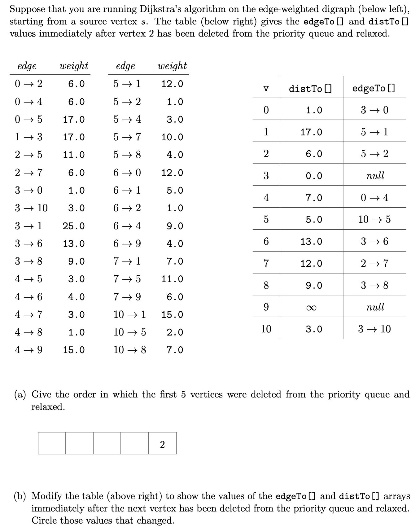
After vertex 2 has been deleted from the PQ, the source to vertex 2 is finalized. According to distTo[2] and edgeTo[2], the distance is $6$ and the vertex pointing to vertex 2 is vertex 5.

According to distTo[3] = 0, the vertex 3 is the source.

Ex 2 (S-T subsets)

Adapted from Algorithms 4.4.25: Given a digraph with positive edge weights, and two distinguished subsets of vertices $S$ and $T$, find a shortest path from any vertex in $S$ to any vertex in $T$. Your algorithm should run in time proportional to $E\log{V}$, in the worst case.

Find two sources first? Or MST? Not sure.

A level

Ex 1 (Transportation)

Problem 6 from Kartik’s Algorithm Worksheet

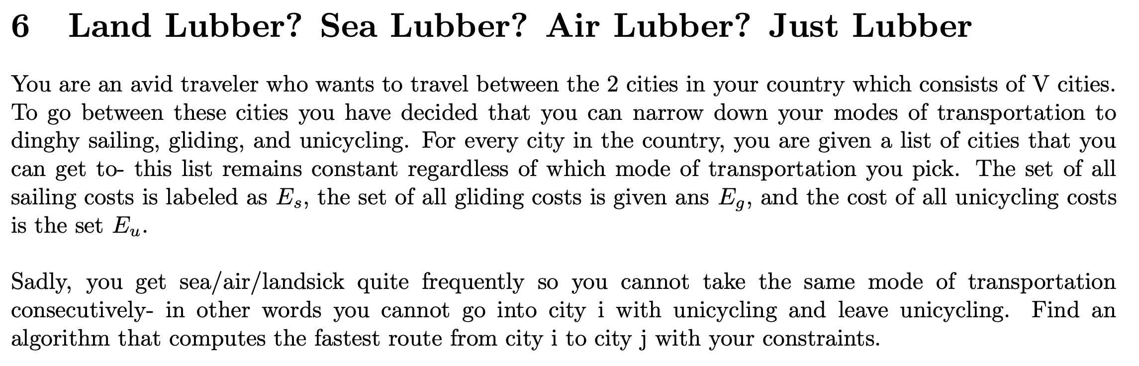
Mark the previous transportation and don’t use the same one when going out.

Ex 2 (Worst-case)

Describe a family of graphs with $V$ vertices and $E$ edges for which the worst-case running time of Dijkstra’s algorithm is achieved.

In worst case, graph will be a complete graph i.e. total edges $E$ would be equal to $\frac{V(V-1)}{2}$ where $V$ is the number of vertices.

Ex 3 (Iterative DFS)

Iterative DFS: Problem 6 from this semester’s discussion worksheet provides a flawed implementation of DFS.

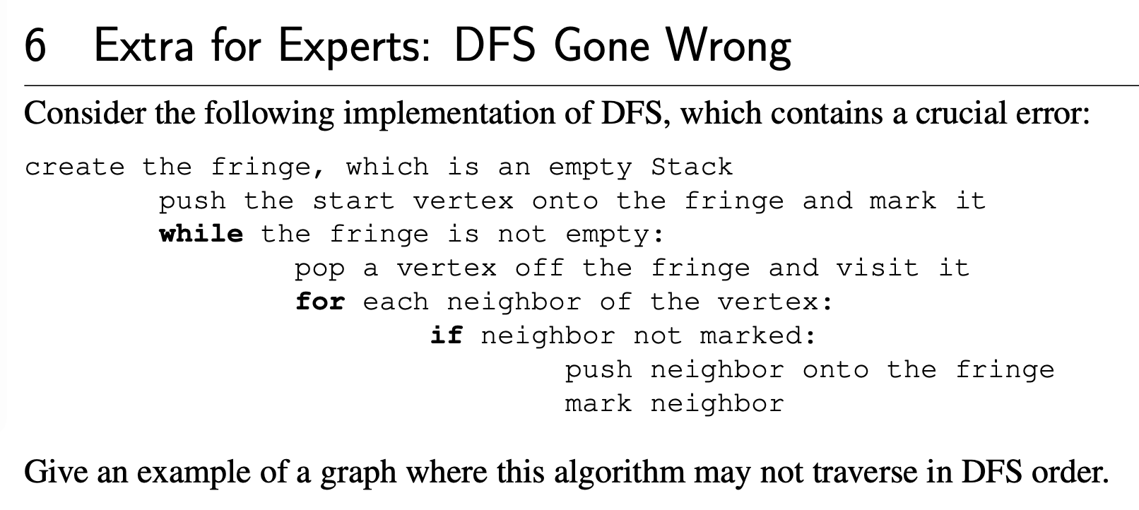
The error is the timing of marking vertices.

Since several copies of a vertex might be in the stack at the same time, we need to check if it is marked before visiting it and its neighbors.

It may visit a vertex twice. For example:

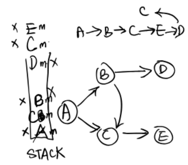
Vertex C is visited twice.

What if we add if not marked after popping a vertex?

More erroneous! Since we marked nodes (like B and C) when looping them from A, we can’t visit B later because it has been marked.

Correct version:

// Using a stack
Initialize the fringe, an empty stack;
  push the starting vertex on the fringe;
  while fringe is not empty:
    pop a vertex off the fringe;
    if vertex is not marked: // since the fringe may contain same nodes
      mark the vertex; // mark here
      visit the vertex;
      for each neighbor of vertex:
        if the neighbor is not marked:
          push the neighbor to fringe.

A+ level

Ex 1 (Monotonic)

Adapted from Algorithms 4.4.34. Give an algorithm to solve the following problem: Given a weighted digraph, find a monotonic shortest path from s to every other vertex. A path is monotonic if the weight of every edge on the path is either strictly increasing or strictly decreasing. The path should be simple (no repeated vertices).

DFS and stop when it is not strictly increasing or decreasing.

Ex 2 (Maximal Increase)

Adapted from Algorithms 4.4.37. Develop an algorithm for finding an edge whose removal causes maximal increase in the shortest-paths length from one given vertex to another given vertex in a given edge-weighted digraph.

For each edge $e$ in the shortest path to destination vertex $t$, calculate the increase if $e$ is not used.

A++ level

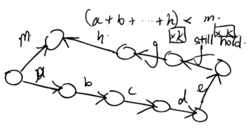
Ex 1 (K-th Shortest Paths)

Idea: Based on the graph with the $m$-th shortest paths, calculate the $m + 1$-th shortest paths.

Assume $G(V,E)$ be the graph.

As for the second shortest paths, an easy approach would be first calculating the shortest path. Let $E’$ be the set of edges belong to this path. For each edge $e$ in $E’$ calculate the shortest path for $G(V, E - e)$.

Minimum Spanning Trees

Warm-up Problem

Problem:

Given an undirected graph, determine if it contains any cycles.

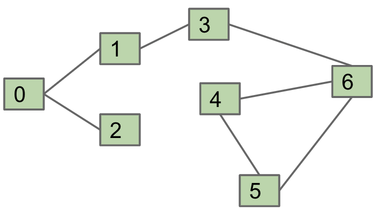
Approach 1: Do DFS from vertex 0 or an arbitrary vertex.

• Keep going until you see a marked vertex.
• Potential danger:
  • 1 looks back at 0 and sees marked.
  • Solution: Just don’t count the node you came from.

Worst case runtime: $O(V + E)$. With some cleverness, can give a tighter bound of $O(V)$.

Approach 2: Use a WeightedQuickUnionUF object.

• For each edge, check if the two vertices are connected.
• If not, union them.
• If so, there is a cycle.

Worst case runtime: $O(V + E\log{V})$ if we have path compression.

Extra problem: (From Discussion 11)

Provide an algorithm that finds the shortest cycle (in terms of the number of edges used) in a directed graph in $O(EV)$ time and $O(E)$ space, assuming $E > V$.

The key idea here is that the shortest cycle involving a particular source vertex $s$ is just the shortest path to a vertex $v$ that has an edge to $s$. We can run BFS on $s$ to find the shortest path to every vertex in the graph. If a vertex $v$ has an edge back to $s$, the length of the cycle involving $s$ and $v$ is one plus distTo(v).

It takes $O(E + V)$ time because it uses BFS and a linear pass through the vertices. Finally, we run BFS on each vertex, so it results in an $V O(E + V) = O(EV + V^2)$.

Since $E > V$, this is still $O(EV)$, because $O(EV + V^2) \leq O(EV + EV) \sim O(EV)$.

Definition

Given an undirected graph, a spanning tree $T$ is a subgraph of $G$, where $T$:

• Is connected.
• Is acyclic. (First two properties make it a tree)
• Includes all vertices. (Spanning)

A minimum spanning tree is a spanning tree of minimum total weight. For example, Directly connecting buildings by power lines.

Applications:

MST vs. SPT

Let’s first compare the MST and SPT.

Is the MST for this graph also a shortest paths tree? If so, using which node as the starting node for this SPT?

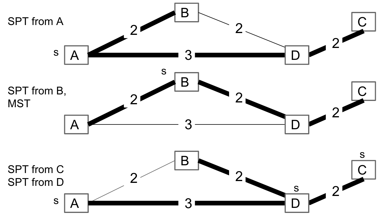
A shortest path tree depends on the start vertex because it tells you how to get from a source to EVERYTHING.

However, there is no source in MST (global property), although sometimes the MST happens to be an SPT for a specific vertex.

So, we may think of a potential algorithm:

• Find the good vertex.
• Run Dijkstra’s.

But, see this example!!!

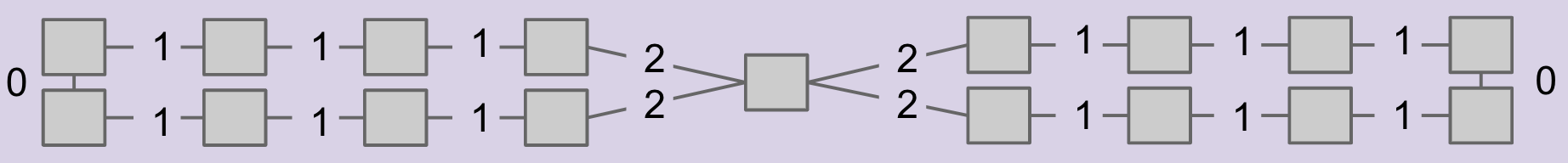
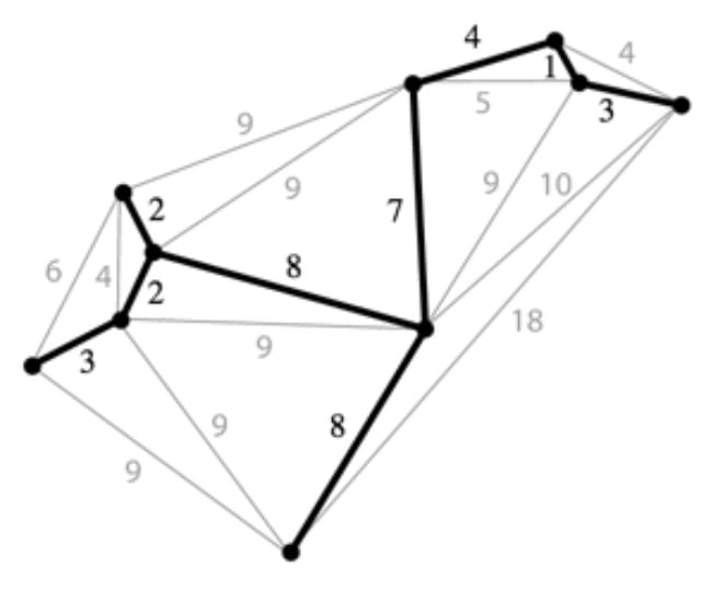
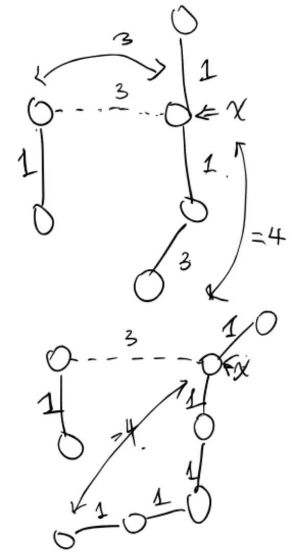
Given a valid MST for the graph below, is there a node whose SPT is also the MST?

It turns out one of the MSTs is as follows:

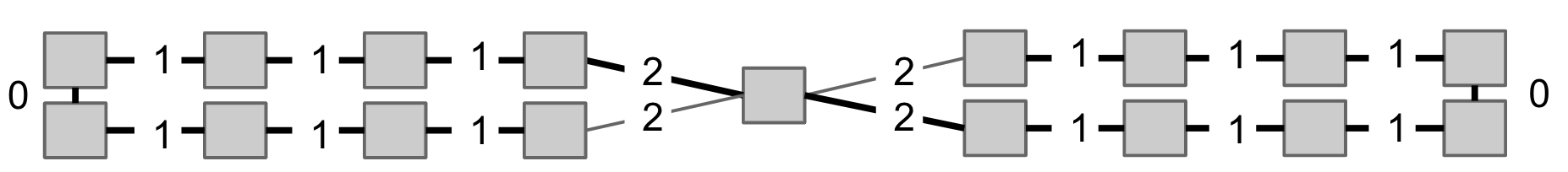
So, again, is there a node whose SPT is also the MST?

Consider the bottom-left and middle nodes.

If we consider the bottom-left node, we have:

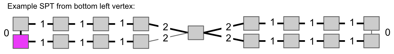
No. The MST must include only two of the 2-weight edges, but the SPT always includes at least three of the 2-weight edges. (at least 4 when the source is the middle node).

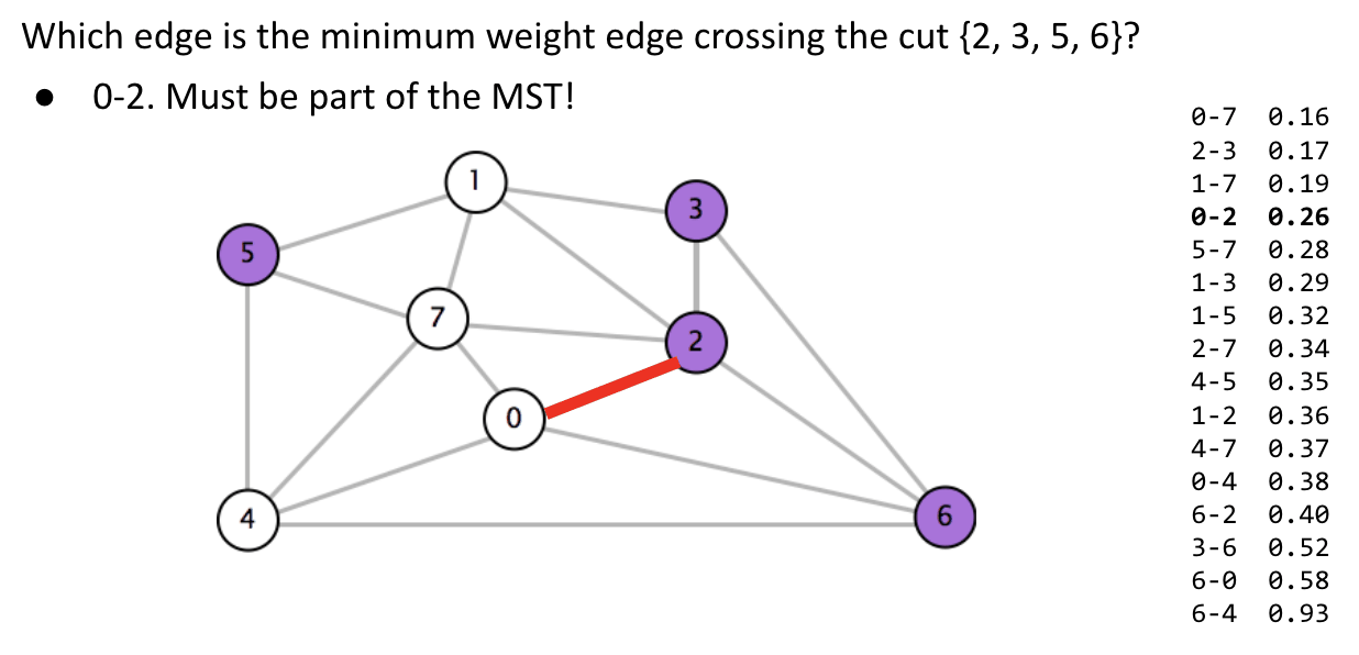
Cut Property

Cut: A cut is an assignment of a graph’s nodes to two non-empty sets. A crossing edge is an edge which connects a node from one set to a node from the other set.

Cut property: Given any cut, minimum weight crossing edge is in the MST.

For example, find the minimum weight crossing edge to connect the nodes from two sets:

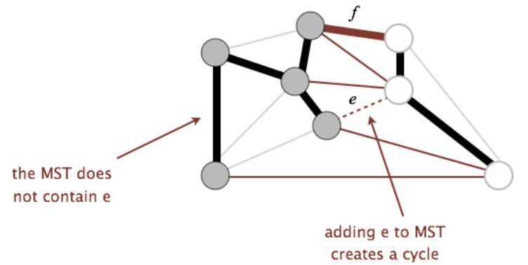
Proof:

Suppose that the minimum crossing edge $e$ were not in the MST.

• Adding $e$ to the MST creates a cycle.
• Some other edge $f$ must also be a crossing edge connecting white and gray nodes.
• Removing $f$ and adding $e$ is a lower weight spanning tree.
• Contradiction (We assume the tree containing $f$ is MST)!

Prim’s Algorithm

Generic MST Finding Algorithm:

Starting no edges in the MST:

• Find a cut that has no crossing edges in the MST.
• Add smallest crossing edge to the MST.
• Repeat until V - 1 edges.

This should work, but need some way of finding a cut with no crossing edges! Random isn’t a very good idea.

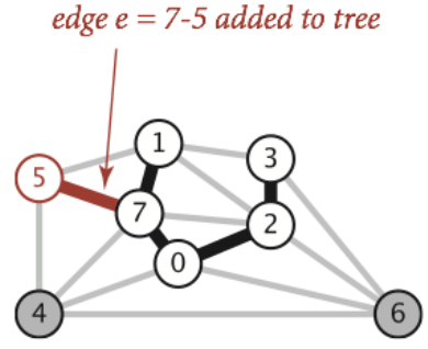
Conceptual Idea

Start from some arbitrary start node:

• Repeatedly add shortest edge (mark black) that has one node inside the MST under construction.
• Repeat until $V - 1$ edges.

Demo: link

Why does Prim’s work? Special case of generic algorithm.

Prim’s algorithm works because at all stages of the algorithm, if we take all the nodes that are part of our MST under construction as one set, and all other nodes as a second set, then this algorithm always adds the lightest edge that crosses this cut, which is necessarily part of the final MST by the Cut property.

• Suppose we add edge $e$ = $v$ -> $w$.
• Side 1 of cut is all vertices connected to our starting vertex (the MST under construction), while side 2 is all the others.
• No crossing edge is black (all connected edges on side 1).
• No crossing edge has lower weight (consider in increasing order).

Note: Sometimes the MST is not unique.

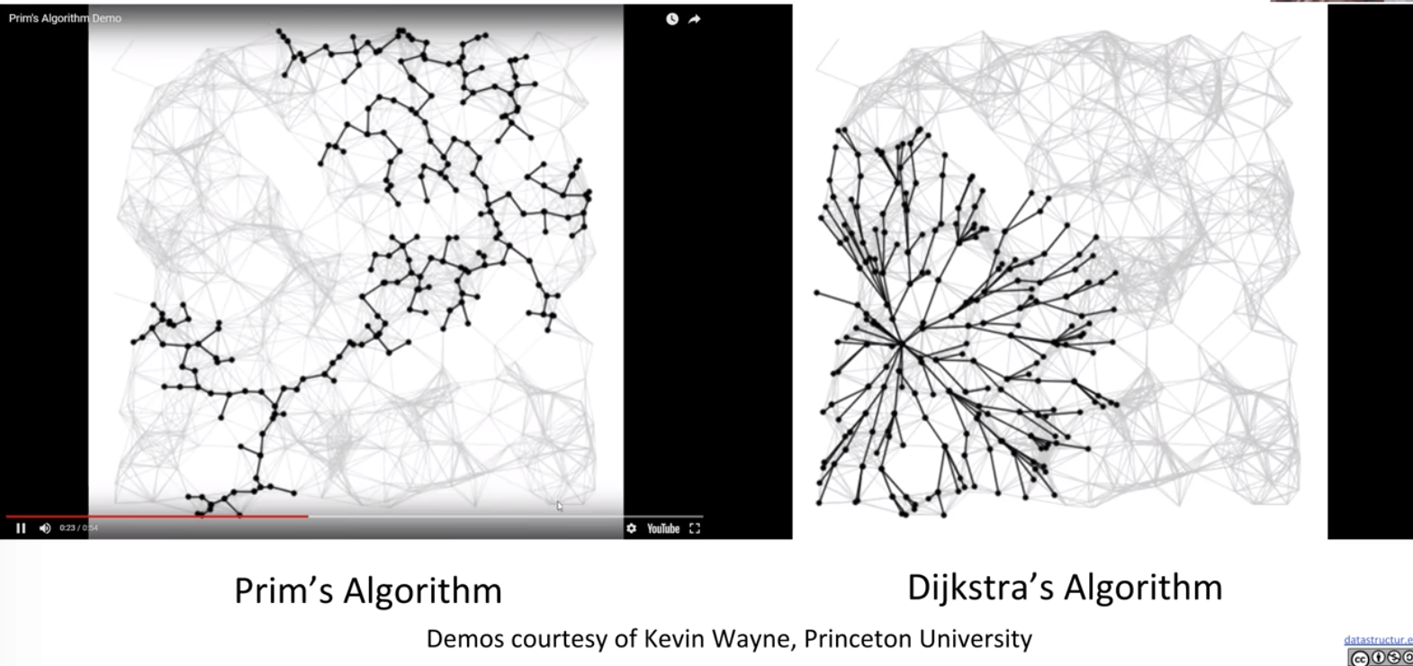
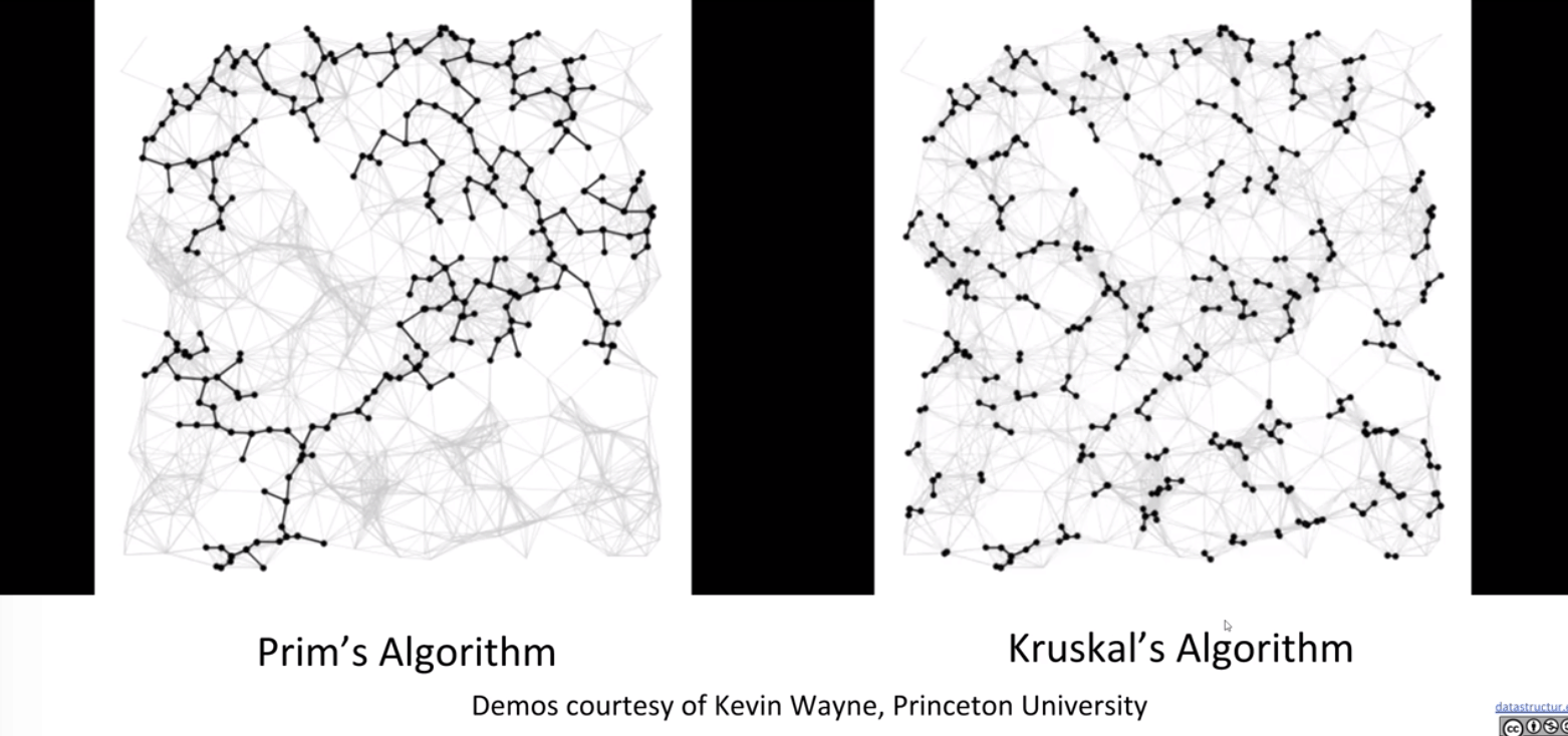
Visualization of Prim’s vs. Dijkstra’s:

Realistic Implementation

The natural implementation of the conceptual version of Prim’s algorithm is highly inefficient, e.g iterating all purple edges.

We can use some cleverness and a PQ to speed things up. The PQ stores the distance between the current MST and the set of the rest vertices

Demo: link

Very interesting.

Note: Vertex removal in this implementation of Prim’s is equivalent to edge addition in the conceptual version of Prim’s.

Prim’s vs. Dijkstra’s

Prim’s and Dijkstra’s algorithms are exactly the same.

Distance:

• Dijkstra’s: Distance from the source.
  • Visit vertices in order of distance from the source.
  • Consider an edge better based on distance to source.
• Prim’s: Distance from the tree.
  • Visit vertices in order of distance from the MST under construction.
  • Consider an edge better based on distance to tree.

Pseudocode

public class PrimMST {
  public PrimMST(EdgeWeightedGraph G) {
    edgeTo = new Edge[G.V()];
    distTo = new double[G.V()];
    marked = new boolean[G.V()];
    fringe = new SpecialPQ<Double>(G.V());

    distTo[s] = 0.0;
    setDistancesToInfinityExceptS(s); // O(V)
    insertAllVertices(fringe); // O(VlogV)
    // Fringe is ordered by distTo

    /* Get vertices in order of distance from the tree */
    while (!fringe.isEmpty()) {
      int v = fringe.delMin();
      marked[v] = true; // v is popped and is the closest (add to MST)
      scan(G, v); // Consider all outgoing edges of v
    }
  }
}

private void scan(EdgeWeightGraph G, v) {
  for (Edge e : G.adj(v)) {
    int w = e.other(v);
    if (marked[w]) continue; // the vertex is in the MST
    if (e.weight() < distTo[w]) {
      distTo[w] = e.weight();
      edgeTo[w] = e;
      pq.decreasePriority(w, distTo[w]); // O(logV)
    }
  }
}

Runtime Analysis

Same as Dijkstra’s runtime.

What is the runtime of Prim’s algorithm?

Assume all PQ operations take $O(\log{V})$ time.

PQ operation count, assuming binary heap based PQ:

• Insertion: $V$, each costing $O(\log{V})$ time.
• Delete-min: $V$, each costing $O(\log{V})$ time.
• Decrease priority: $E$, each costing $O(\log{V})$ time.

Overall runtime: $O(V\log{V} + V\log{V} + E\log{V}) = O((V + E)\log{V})$.

Assuming $E > V$, this is just $O(E\log{V})$.

Kruskal’s Algorithm

Conceptual Idea

Neat property: Relatively easy and intuitive.

Initially mark all edges gray.

• Consider edges in increasing order of weight.
• Add edge to MST (mark black) unless doing so creates a cycle.
• Repeat until $V-1$ edges.

Why does it work? Special case of generic MST algorithm.

For every time you consider the smallest-weight edge, there’s some cut for which the cut property proves that the addition of that edge will actually be valid.

Consider side 1 of cut is all vertices connected to $v$, side 2 is everything else.

Note: It’s not fully connected at all time, unlike the invariant of Prim’s Algorithm.

Demo: link

Realistic Implementation

Insert all edges into PQ. Repeat: remove smallest weight edge. Add to MST if no cycle created.

• Use a PQ (fringe) to store all edges.
• Use a WQU (Weighted Quick Union with Path Compression) to see if cycle is created (using isConnected(v, w)).
• Use a MST to store the tree.

Demo: link

Prim’s vs. Kruskal’s

Guarantee the same weight.

Pseudocode

public class KruskalMST {
  private List<Edge> mst = new ArrayList<>();

  public KruskalMST(EdgeWeightedGraph G) {
    for (Edge e : G.edges()) { // E times
      pq.insert(e); // O(logE)
    } // If we have a pre-sorted list
      // If using bottom-up heapification => O(E)
    WeightedQuickUnionPC uf = new WeightedQuickUnionPC(G.V());

    // In case of disconnected components
    // Assume E > V
    while (!pq.isEmpty() && mst.size() < G.V() - 1) { // E times
      Edge e = pq.delMin(); // O(logE)
      int v = e.from();
      int w = e.to();
      if (!uf.isConnected(v, w)) { // O(log*V) for E times
        uf.union(v, w); // O(log*V) but only for V times
        mst.add(e); // O(1)
      }
    }
  }
  // Insert + delMin + isConnected + union + add
  // O(ElogE + ElogE + Elog*V + Vlog*V + V)
  // = O(ElogE + Elog*V + Vlog*V + V)
  // = O(ElogE)
  //
  // If using a pre-sorted list: (no need to use PQ)
  // Sorting takes O(ElogE)
  // O(E + E + Elog*V + Vlog*V + V)
  // = O(Elog*V)
}

Runtime Analysis

See the pseudocode for details.

Note: $\log^{*}{V}$ is the iterative logarithm which is less than 5.

• Assume all PQ operations take $O(\log{V})$ time.
• Assume all WQU operations take $O(\log^{*}{V})$ time.

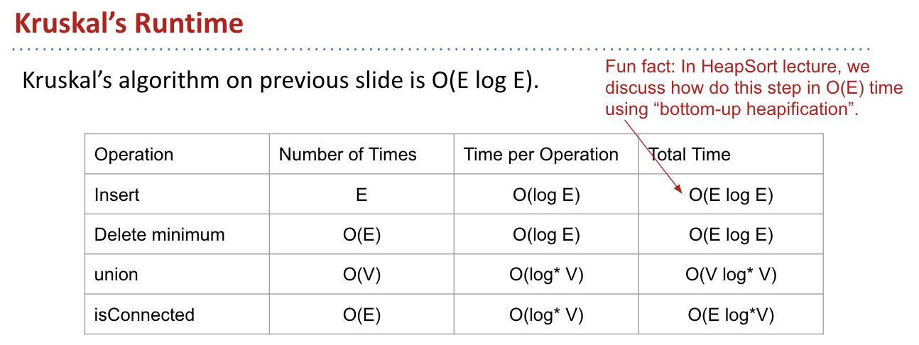
Note: If we use a pre-sorted list of edges (instead of PQ), then we can simple iterate through the list in $O(E)$ time. So overall runtime is O(E + Vlog* V + Elog* V) = $O(E\log^{*}{V})$.

So far, the runtime summary:

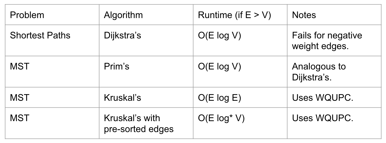
We can see Prim’s is a little bit faster than Kruskal’s, but it is negligible. Kruskal is little bit easier to implement.

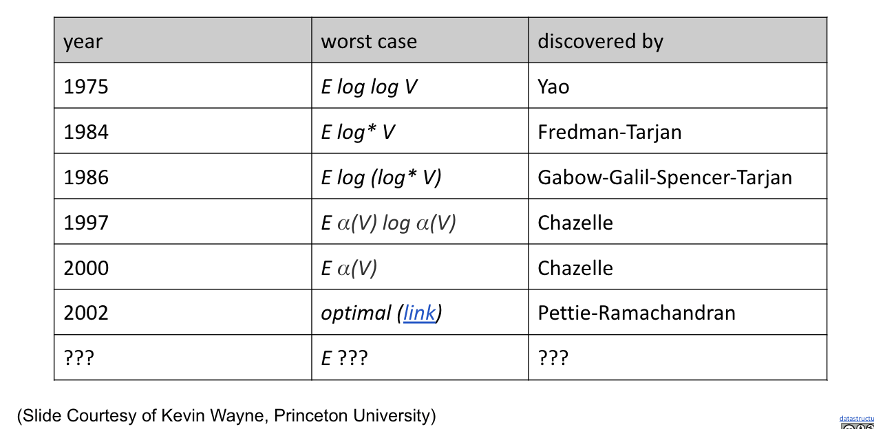
Question: Can we do better than $O(E\log^{*}{V})$?

State of the Art Compare-Based MST Algorithms:

Ex (Guide)

C level

Ex 1 (Directed)

Would Kruskal or Prim’s algorithm work on a directed graph?

Can Prim’s and Kruskal’s algorithm be used on a directed graph to generate a Minimal Spanning Tree?

No. Prim’s and Kruskal’s algorithm works only for undirected graphs. For directed graphs, the equivalent notion of a spanning tree is spanning arborescence. A minimum weight spanning arborescence can be found using Edmonds' algorithm.

Ex 2 (Add Constant)

True or false: Adding a constant to every edge weight does not change the solution to the MST problem (assume unique edge weights).

True. Consider Kruskal's Algorithm. The order of the list is still the same.

Ex 3 (Multiply Constant)

True or false: Multiplying all edges weights with a constant does not change the solution to the MST problem (assume unique edge weights).

False. Consider the constant is $0$ or negative numbers.

Ex 4 (Other True/False)

True or false: It is possible that the only Shortest Path Tree is the only Minimum Spanning Tree.

True. A list.

True or false: Prim’s Algorithm and Kruskal’s Algorithm will always return the same result.

False. Only the total weight is guaranteed.

B level

Ex 1 (Remain MST?)

Problem 3 from Princeton’s Fall 2009 final (part d is pretty hard).

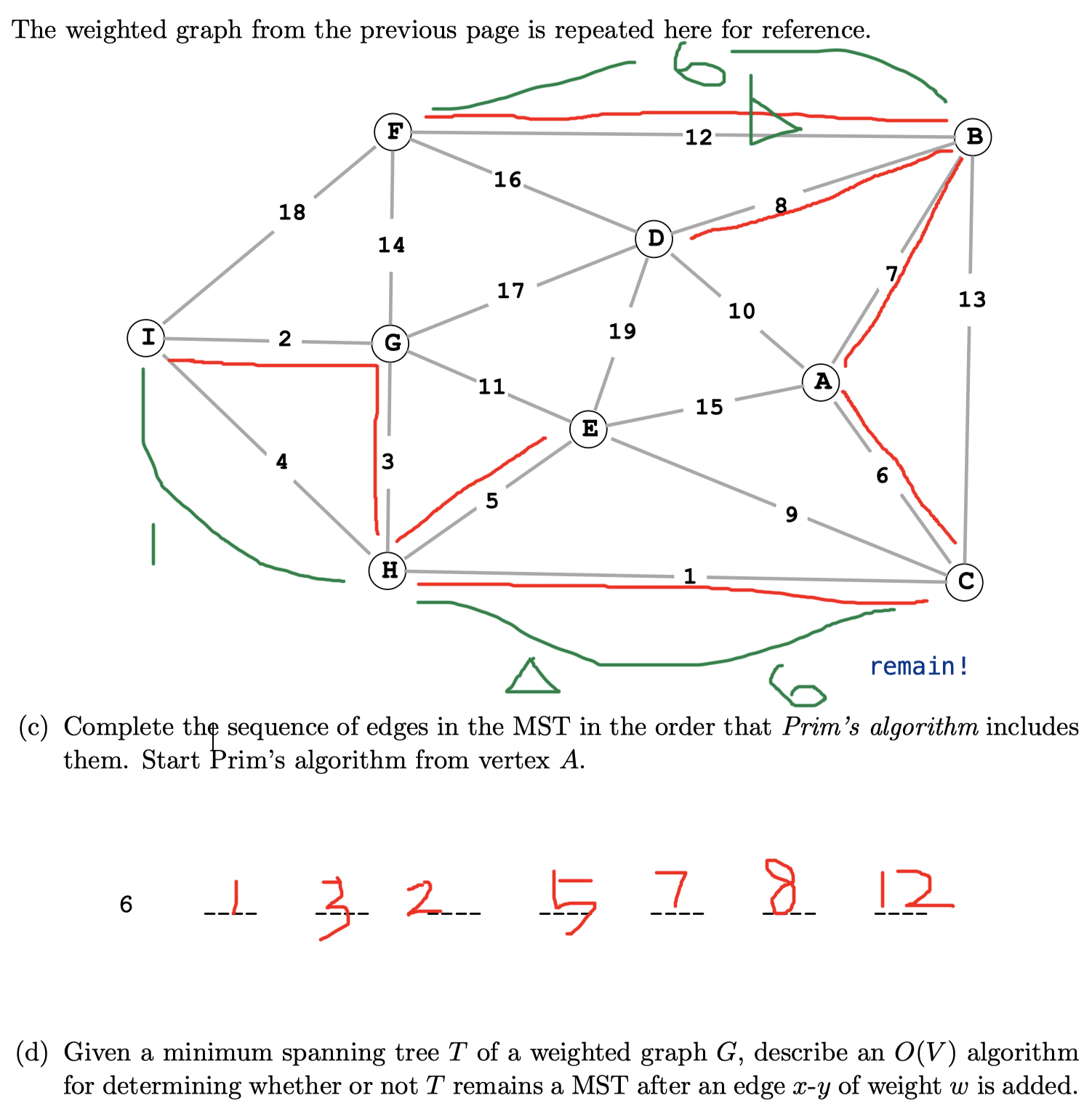
(d) Find the path (only one) between $x$ and $y$ in $T$, which takes $O(V)$ time using DFS because there are only $V-1$ edges in $T$. If $w$ is greater than or equal to the current weight of every edge, $T$ remains an MST.

• If otherwise, that is, any edge on the path has weight greater than $w$, we can decrease the weight of $T$ by swapping the largest weight edge on the path with $x-y$. Thus, $T$ does not remain an MST.
  • This one is confusing. I think it depends on where the largest edge is (see the edges in green).
  • I think T does not remain an MST. But if we swap the largest path in the cycle with $x-y$, it generates a new valid MST.
• If $w$ is greater than or equal to the weight of every edge on the path, then the cycle property asserts that $x-y$ is not in some MST (because it is the largest weight edge on the cycle consisting of the path from $x$ to $y$ pluse the edge $x-y$). Thus, $T$ remains an MST.

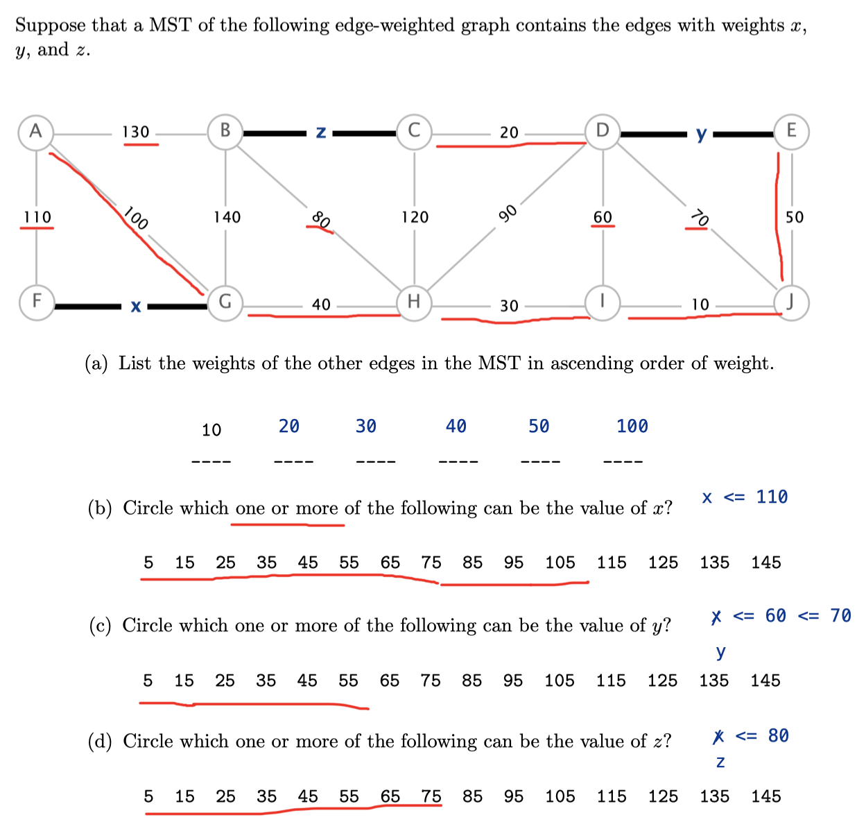
Ex 2 (x-y-z)

Problem 4 from Princeton’s Fall 2012 final.

Ex 3 (Belong?)

Adapted from Algorithms 4.3.12. Suppose that a graph has distinct edge weights.

• Does its shortest edge have to belong to the MST? Can its longest edge belong to the MST?
• Does a min-weight edge on every cycle have to belong to the MST?

Prove your answer to each question or give a counterexample.

Its shortest edge has to belong to the MST! Consider using Kruskal’s Algorithm to build the MST. We always add the shortest edge first and in every case the first shortest path will not incur a cycle since there is no path in the MST at first.

It longest edge can belong to the MST, e.g number of edges $E = V - 1$.

Ex 4 (Closer?)

Adapted from Algorithms 4.3.20. True or false: At any point during the execution of Kruskal’s algorithm, each vertex is closer to some vertex in its subtree than to any vertex not in its subtree. Prove your answer.

True. Since it is some vertex, it is true. The edges connecting these vertices to that point have always been added to the MST before any vertex (e.g vertex 3) not in its subtree.

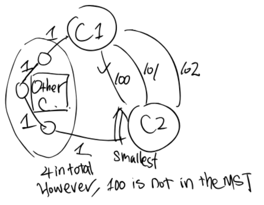
Ex 5 (Any Two Components)

True or False: Given any two components that are generated as Kruskal’s algorithm is running (but before it has completed), the smallest edge connecting those two components is part of the MST.

False.

Ex 6 (Total Weight)

Problem 11 from my Fall 2014 final.

Assume that all edge weights are unique, and may be negative, zero, or positive.

True or False: The total weight of an MST of an undirected graph is always less than or equal to the total weight of any shortest-path tree for that graph.

True. Since a shortest path is one of the spanning trees which contains all vertices of a connected graph, its total weight must be less than an MST.

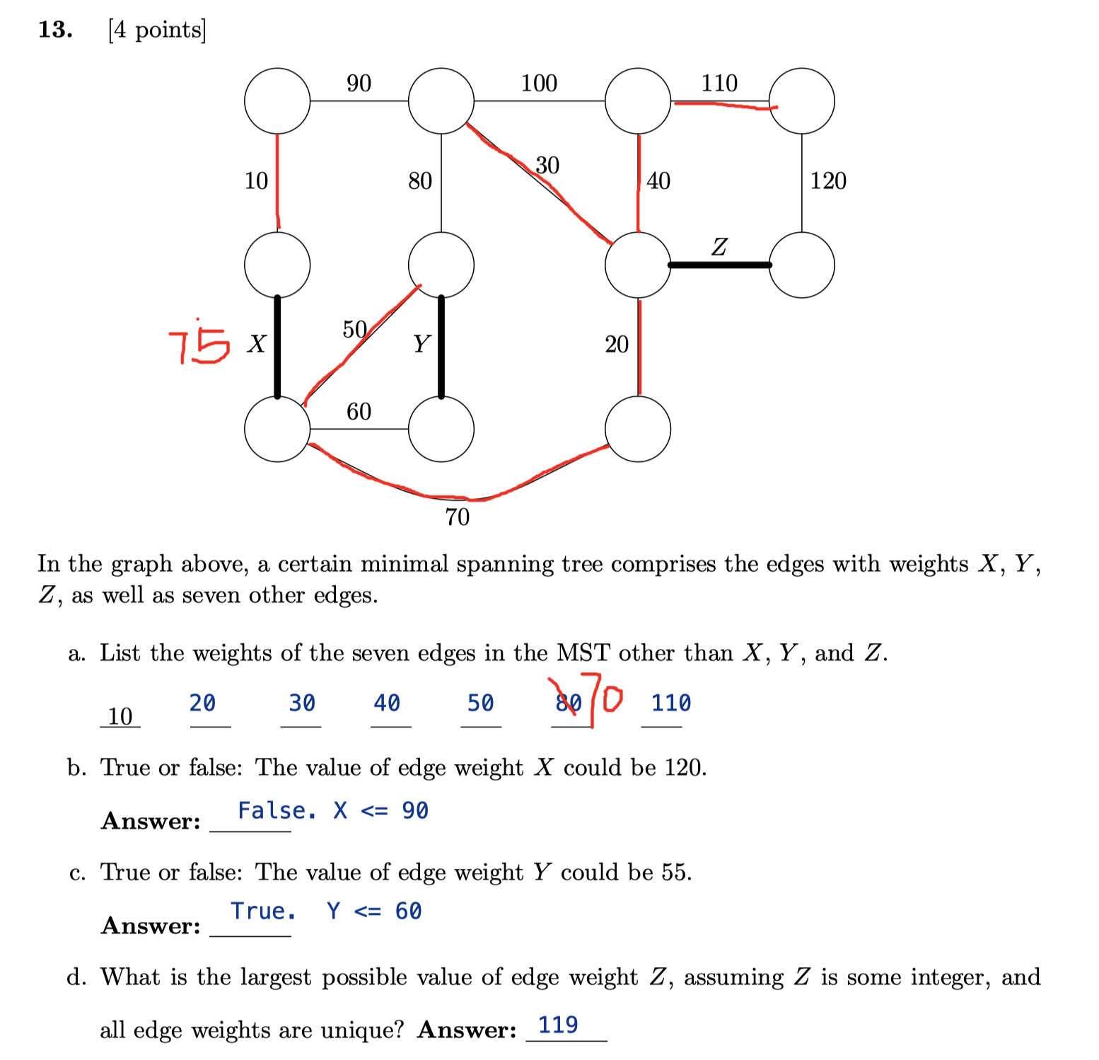
Ex 7 (x-y-z)

Problem 13 from my Fall 2014 final.

Ex 8 (Product MST)

How would you find the Minimum Spanning Tree where you calculate the weight based off the product of the edges rather than the sum. You may assume that edge weights are > 1.

We can still use the two algorithms. But we need to change the weight of each edge to log value first.

$$\log{(w_1 \times w_2 \times \dots \times w_{E})} = \log{w_1} + \log{w_2} + \dots + \log{w_E} $$

A level

Ex 1 (Critical Edge)

Adapted from Textbook 4.3.26: An MST edge whose deletion from the graph would cause the MST weight to increase is called a critical edge. Show how to find all critical edges in a graph in time proportional to $E\log{E}$.

Note: This question assumes that edge weights are not necessarily distinct (otherwise all edges in the MST are critical).

For each edge $x-y$ in the MST, temporarily remove vertex $x$ or $y$ from the WQU. If $x$ are $y$ are still connected, it means there is a cycle such that $x-y$ can be replaced.

For each the edges of $x$ or $y$, if there is any edge with the same weight as the edge in the MST, it is not critical. It check $2E$ times in the worst case.

Ex (Examprep 10)

Ex 1 (Distinct Weights in SP)

True or False: If all edges have distinct weights, the shortest path between any two vertices is unique.

Ex 2 (Faster SP Algorithm)

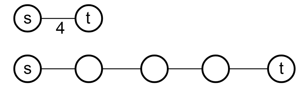
Design an efficient algorithm for the following problem: Given a weighted, undirected, and connected graph $G$, where the weights of every edge in $G$ are all integers between $1$ and $10$, adn a starting vertex $s$ in $G$, find the distance from $s$ to every other vertex in the graph (where the distance between two vertices is defined as the weight of the shortest path connecting them).

You algorithm must run asymptotically faster than Dijkstra’s.

• $\Theta(|V| + |E|)$. Convert $x$-weight edge to $x-1$ vertices with 1-weight edges connecting them. Then use BFS to get the shortest path.
  

• Modify the PQ to return minimum values faster. Create 11 buckets with linked lists and each edge of a specific weight corresponds to a particular bucket.

Reference: Dial’s Algorithm